<?xml version="1.0" encoding="utf-8"?><feed xmlns="http://www.w3.org/2005/Atom" xml:lang="en-IN"><generator uri="https://jekyllrb.com/" version="3.10.0">Jekyll</generator><link href="https://wealthprimer.in/feed.xml" rel="self" type="application/atom+xml" /><link href="https://wealthprimer.in/" rel="alternate" type="text/html" hreflang="en-IN" /><updated>2026-10-03T16:05:45+05:30</updated><id>https://wealthprimer.in/feed.xml</id><title type="html">Wealth Primer</title><subtitle>Financial education, one concept at a time — fundamental analysis, technical analysis, mutual funds, and financial jargon explained for Indian retail investors. Educational content only, not investment advice.</subtitle><author><name>Himanshu Gupta</name></author><entry><title type="html">Alpha: the return that’s left after the market is accounted for</title><link href="https://wealthprimer.in/2026/10/03/alpha/" rel="alternate" type="text/html" title="Alpha: the return that’s left after the market is accounted for" /><published>2026-10-03T09:00:00+05:30</published><updated>2026-10-03T09:00:00+05:30</updated><id>https://wealthprimer.in/2026/10/03/alpha</id><content type="html" xml:base="https://wealthprimer.in/2026/10/03/alpha/"><![CDATA[<h2 id="what-alpha-means">What alpha means</h2>

<p><strong>Alpha</strong> is the return an investment earned <em>beyond</em> what you’d have expected
given the risk it took. It’s the number every active fund manager is
implicitly claiming to produce, and the number this blog’s mutual fund series
has so far avoided using — because most of what gets called alpha is
something else wearing the name.</p>

<p>There are two very different things people mean by it:</p>

<ol>
  <li><strong>Raw excess return</strong> — the investment’s return minus the benchmark’s.
Simple, and usually what a factsheet or a headline means.</li>
  <li><strong>Jensen’s alpha</strong> — the return minus what CAPM (the Capital Asset
Pricing Model) says the investment
<em>should</em> have earned, given its <a href="/2026/10/02/beta/">beta</a>.
This is the one that deserves the name.</li>
</ol>

<p>The gap between the two is the whole lesson.</p>

<h2 id="the-formula">The formula</h2>

<div class="language-plaintext highlighter-rouge"><div class="highlight"><pre class="highlight"><code>Raw excess return  =  R_investment − R_benchmark

Jensen's alpha     =  R_investment − [ R_f + β × (R_benchmark − R_f) ]

where  R_f  = risk-free rate
       β    = the investment's beta against that benchmark
</code></pre></div></div>

<p>The bracket is CAPM’s expected return: the risk-free rate, plus beta times
the market’s excess return. A stock with a beta of 2 that returned 20% in a
year the market returned 10% has <em>no</em> alpha — doubling the market is exactly
what a beta of 2 is supposed to do.</p>

<h2 id="worked-example-britannia-two-years">Worked example: Britannia, two years</h2>

<p>Daily closes from 1 April 2024 to 30 March 2026, the same series as the <a href="/2026/10/02/beta/">beta post</a>
(whose first daily return falls on the next trading day).
Risk-free rate 6.5%, the illustrative G-Sec (Government of India
bond) yield used throughout the
<a href="/2026/09/28/wacc-cost-of-capital/">WACC post</a>. Historical data, for
illustration only.</p>

<table>
  <thead>
    <tr>
      <th> </th>
      <th style="text-align: right"> </th>
    </tr>
  </thead>
  <tbody>
    <tr>
      <td>Britannia, annualised return</td>
      <td style="text-align: right">5.27%</td>
    </tr>
    <tr>
      <td>Nifty 50 (price index), annualised</td>
      <td style="text-align: right">-0.29%</td>
    </tr>
    <tr>
      <td><strong>Raw excess return</strong></td>
      <td style="text-align: right"><strong>5.56 pp a year</strong></td>
    </tr>
    <tr>
      <td>Britannia’s beta over the window</td>
      <td style="text-align: right">0.42</td>
    </tr>
    <tr>
      <td>CAPM expected return: 6.5 + 0.42 × (−0.29 − 6.5)</td>
      <td style="text-align: right">3.65%</td>
    </tr>
    <tr>
      <td><strong>Jensen’s alpha</strong></td>
      <td style="text-align: right"><strong>1.62 pp a year</strong></td>
    </tr>
  </tbody>
</table>

<p>Same stock, same two years: the headline says Britannia beat the market by
5.56 points a year; the risk-adjusted version says 1.62. The difference
is that the Nifty had a poor two years — the price index actually <em>fell</em>
slightly — and a stock with a beta of 0.42 was <em>expected</em> to fall less. Most
of the “outperformance” is just low beta doing what low beta does in a weak
market. Reverse the market and the same low beta would have made Britannia
look like a laggard.</p>

<p>One honest caveat on the inputs. Both returns here are <em>price-only</em>:
Britannia’s share price and the Nifty 50 price index, with dividends left
out, because a total return index series isn’t in this post’s data. That’s
the very mistake the next section warns about. In the raw comparison the two
missing dividend streams partly cancel. In the CAPM line they don’t: the
risk-free rate is a full yield, but the market return it’s compared with is
missing its dividends, so the market’s excess return is understated. Treat
the alpha figure as rough — it illustrates the method, not a precise
measurement.</p>

<p>Neither figure says anything about Britannia’s prospects. It’s two years of
price history, and the <a href="/2026/10/02/beta/">beta post</a> already
showed that the beta itself moved from 0.29 to 0.55 across those two years —
so the alpha number inherits every bit of that instability.</p>

<h2 id="the-fake-alpha-in-every-index-fund-factsheet">The fake alpha in every index fund factsheet</h2>

<p>Here is a more instructive example. Take the UTI Nifty 50 Index Fund (regular plan) — a
passive fund whose entire job is to <em>match</em> the index — and compute its
calendar-year return minus the Nifty 50 price index:</p>

<table>
  <thead>
    <tr>
      <th>Year</th>
      <th style="text-align: right">Fund</th>
      <th style="text-align: right">Nifty 50 (price)</th>
      <th style="text-align: right">Difference</th>
    </tr>
  </thead>
  <tbody>
    <tr>
      <td>2016</td>
      <td style="text-align: right">4.0%</td>
      <td style="text-align: right">3.01%</td>
      <td style="text-align: right">+0.99 pp</td>
    </tr>
    <tr>
      <td>2017</td>
      <td style="text-align: right">29.68%</td>
      <td style="text-align: right">28.65%</td>
      <td style="text-align: right">+1.03 pp</td>
    </tr>
    <tr>
      <td>2018</td>
      <td style="text-align: right">4.26%</td>
      <td style="text-align: right">3.15%</td>
      <td style="text-align: right">+1.11 pp</td>
    </tr>
    <tr>
      <td>2019</td>
      <td style="text-align: right">13.25%</td>
      <td style="text-align: right">12.02%</td>
      <td style="text-align: right">+1.22 pp</td>
    </tr>
    <tr>
      <td>2020</td>
      <td style="text-align: right">15.5%</td>
      <td style="text-align: right">14.9%</td>
      <td style="text-align: right">+0.6 pp</td>
    </tr>
    <tr>
      <td>2021</td>
      <td style="text-align: right">25.2%</td>
      <td style="text-align: right">24.12%</td>
      <td style="text-align: right">+1.08 pp</td>
    </tr>
    <tr>
      <td>2022</td>
      <td style="text-align: right">5.33%</td>
      <td style="text-align: right">4.33%</td>
      <td style="text-align: right">+1.0 pp</td>
    </tr>
    <tr>
      <td>2023</td>
      <td style="text-align: right">20.89%</td>
      <td style="text-align: right">20.03%</td>
      <td style="text-align: right">+0.86 pp</td>
    </tr>
    <tr>
      <td>2024</td>
      <td style="text-align: right">9.64%</td>
      <td style="text-align: right">8.8%</td>
      <td style="text-align: right">+0.84 pp</td>
    </tr>
    <tr>
      <td>2025</td>
      <td style="text-align: right">11.57%</td>
      <td style="text-align: right">10.51%</td>
      <td style="text-align: right">+1.06 pp</td>
    </tr>
  </tbody>
</table>

<p>Ten years, ten positive numbers, averaging <strong>+0.98 pp a year</strong>.
Sources: fund NAV from AMFI via mfapi.in; index from Yahoo Finance. Data to
31 March 2026.</p>

<p>An index fund with a decade of positive “alpha” is obviously nonsense — and it
is, because the benchmark is wrong. The <strong>price index (PRI)</strong> ignores the
dividends the fifty companies pay; the fund receives and reinvests them. That
one-point gap is roughly the Nifty’s dividend yield minus the fund’s expense
ratio. Against the <strong>total return index (TRI)</strong>, which includes dividends, the
same fund would likely show a <em>small negative</em> number most years — the expense ratio
and tracking error, which is what an index fund is supposed to show.</p>

<p>This is exactly why the
<a href="/2026/10/02/benchmarks-and-comparing-like-with-like/">benchmarks post</a>
insisted on comparing like with like, and why SEBI has required funds to
benchmark against TRI since February 2018. Before that, a lot of Indian
active-fund “alpha” was this dividend gap.</p>

<details>
  <summary>🧒 Explain it like I'm 10 <em>(optional — skip if this is already clear)</em></summary>

  <p>Your friend says she’s a better runner than you because she finished the race
30 seconds ahead. But she started 30 seconds before you did. Once you account
for the head start, she didn’t beat you at all.</p>

  <p>Alpha is the finishing time <em>after</em> subtracting head starts. Beta is one head
start (some runners just get a tailwind when the whole field does). Dividends
the benchmark forgot to count are another.</p>

</details>

<h2 id="common-mistakes">Common mistakes</h2>

<ul>
  <li><strong>Calling excess return “alpha”.</strong> Excess return over a benchmark is a
fact. Alpha is that fact with the risk taken to earn it subtracted out. A
high-beta fund in a bull market has lots of the first and often none of the
second.</li>
  <li><strong>Benchmarking against a price index.</strong> It manufactures about a point a
year of alpha out of dividends. Always check whether a comparison uses PRI
or TRI.</li>
  <li><strong>Reading alpha over a short window.</strong> Two years of Britannia produced an
alpha estimate built on a beta that nearly doubled inside the window. Alpha
needs a horizon long enough for the beta to mean something, and even then
the standard error is usually larger than the estimate.</li>
  <li><strong>Assuming past alpha persists.</strong> The consistency of the index fund’s
“alpha” above is the exception — it’s a structural artefact. Genuine
manager alpha is hard to find at all: S&amp;P’s
<a href="https://www.spglobal.com/spdji/en/documents/spiva/spiva-india-scorecard-year-end-2025.pdf">SPIVA India Year-End 2025 scorecard</a>
found about 76% of Indian active large-cap funds trailed their benchmark
over the ten years to December 2025. Finding it <em>and</em> expecting it to
continue is harder still.</li>
</ul>

<p><strong>Takeaway:</strong> alpha is what’s left of a return after the benchmark <em>and</em> the
beta are accounted for. Britannia’s 5.56-point lead over a weak Nifty shrinks
to 1.62 once its low beta is credited — and an index fund’s decade of
“outperformance” over the price index is dividends, not skill.</p>]]></content><author><name>{&quot;twitter&quot;=&gt;&quot;wealthprimer_in&quot;}</name></author><summary type="html"><![CDATA[Alpha is return beyond what beta and the benchmark predict. Britannia's 5.6-point lead over the Nifty is 1.6 after beta; an index fund's alpha is dividends.]]></summary><media:thumbnail xmlns:media="http://search.yahoo.com/mrss/" url="https://wealthprimer.in/assets/og/alpha.png" /><media:content medium="image" url="https://wealthprimer.in/assets/og/alpha.png" xmlns:media="http://search.yahoo.com/mrss/" /></entry><entry><title type="html">How to read a candlestick chart: open, high, low, close</title><link href="https://wealthprimer.in/2026/10/03/reading-a-candlestick-chart/" rel="alternate" type="text/html" title="How to read a candlestick chart: open, high, low, close" /><published>2026-10-03T09:00:00+05:30</published><updated>2026-10-03T09:00:00+05:30</updated><id>https://wealthprimer.in/2026/10/03/reading-a-candlestick-chart</id><content type="html" xml:base="https://wealthprimer.in/2026/10/03/reading-a-candlestick-chart/"><![CDATA[<h2 id="why-not-just-a-line">Why not just a line?</h2>

<p>The <a href="/2026/10/02/what-technical-analysis-is/">last post</a> showed Britannia’s
price as a simple line — one dot per day, joined up. It’s readable, and it
throws away most of the information.</p>

<p>A line chart plots the closing price. But a trading day isn’t one number. The
stock opened somewhere, traded up to some highest point, down to some lowest
point, and closed somewhere else. A day that opened at ₹5,000, spiked to
₹5,300, collapsed to ₹4,900 and closed at ₹5,010 looks, on a line chart,
almost identical to a day that drifted quietly from ₹5,000 to ₹5,010.</p>

<p>Those were not the same day. <strong>Candlesticks</strong> — developed by Japanese rice
traders in the 1700s and popularised in the West by Steve Nison in the
1990s — show all four prices in a single bar.</p>

<h2 id="the-anatomy">The anatomy</h2>

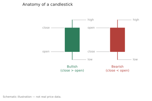
<p><img src="/assets/charts/ta-candle-anatomy.svg" alt="Anatomy of a candlestick" /></p>

<p>Schematic illustration — not real price data.</p>

<p>Each candle has two parts:</p>

<table>
  <thead>
    <tr>
      <th>Part</th>
      <th>What it shows</th>
    </tr>
  </thead>
  <tbody>
    <tr>
      <td><strong>Body</strong> (the thick rectangle)</td>
      <td>The range between the open and the close</td>
    </tr>
    <tr>
      <td><strong>Wicks</strong> (the thin lines, also called shadows)</td>
      <td>The extremes — the high above, the low below</td>
    </tr>
  </tbody>
</table>

<p>And the colour tells you the direction:</p>

<ul>
  <li><strong>Green (or white/hollow)</strong> — the close was <em>above</em> the open. Buyers ended
the session in control.</li>
  <li><strong>Red (or black/filled)</strong> — the close was <em>below</em> the open. Sellers did.</li>
</ul>

<p>That’s the whole notation. A long body means the open and close were far
apart — a decisive session. A short body means they finished near each other,
whatever happened in between. Long wicks mean the price went somewhere and
came back.</p>

<details>
  <summary>🧒 Explain it like I'm 10 <em>(optional — skip if this is already clear)</em></summary>

  <p>Think of a tug-of-war that lasts all day.</p>

  <p>The <strong>body</strong> shows where the rope started and where it ended up. If it ended
up on the buyers’ side, the candle is green. If the sellers dragged it their
way, it’s red.</p>

  <p>The <strong>wicks</strong> show how far the rope got pulled at the furthest moments,
before being hauled back. A really long wick upward means the buyers got the
rope almost all the way over — and then lost it again before the whistle.</p>

  <p>A line chart only tells you where the rope finished. Candles tell you how
hard the fight was.</p>

</details>

<h2 id="reading-real-candles">Reading real candles</h2>

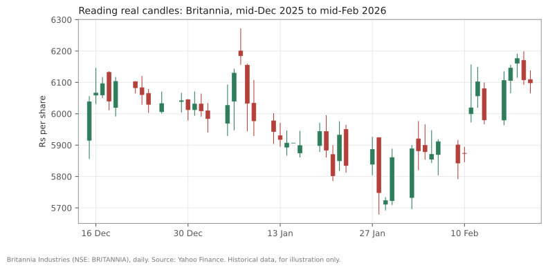
<p>Here’s Britannia through the turn of 2026 — two months of real trading days:</p>

<p><img src="/assets/charts/ta-candles-real.svg" alt="Britannia candlestick chart, December 2025 to February 2026" /></p>

<p>Britannia (NSE: BRITANNIA), daily, mid-December 2025 to mid-February 2026.
Source: <a href="https://finance.yahoo.com/quote/BRITANNIA.NS/history/">Yahoo Finance</a>. Historical data, for
illustration only.</p>

<p>Some things you can read straight off it that a line chart would have hidden:</p>

<ul>
  <li><strong>Long upper wicks near the highs.</strong> Several sessions in early January
pushed up and closed well below where they’d reached. Buyers got the price
up there; it didn’t stay.</li>
  <li><strong>Alternating colours in the middle.</strong> Long stretches of green-red-green-red
with small bodies — sessions that opened and closed near each other. That’s
a market with no settled view.</li>
  <li><strong>The occasional long body.</strong> A few sessions ran decisively one way. Those
are days when something happened.</li>
</ul>

<h2 id="the-single-candle-shapes-worth-knowing">The single-candle shapes worth knowing</h2>

<p>A handful of individual candles have names. They describe the shape, and the
usual interpretation attached to each is much softer than most sources admit.</p>

<table>
  <thead>
    <tr>
      <th>Shape</th>
      <th>Looks like</th>
      <th>Usual reading</th>
    </tr>
  </thead>
  <tbody>
    <tr>
      <td><strong>Doji</strong></td>
      <td>Almost no body — open ≈ close</td>
      <td>Indecision; neither side won</td>
    </tr>
    <tr>
      <td><strong>Hammer</strong></td>
      <td>Small body at the top, long lower wick</td>
      <td>Sellers pushed down, buyers pulled it back</td>
    </tr>
    <tr>
      <td><strong>Shooting star</strong></td>
      <td>Small body at the bottom, long upper wick</td>
      <td>Buyers pushed up, sellers pulled it back</td>
    </tr>
    <tr>
      <td><strong>Marubozu</strong></td>
      <td>Long body, almost no wicks</td>
      <td>One-sided conviction all session</td>
    </tr>
  </tbody>
</table>

<p>And two-candle combinations:</p>

<table>
  <thead>
    <tr>
      <th>Shape</th>
      <th>Looks like</th>
      <th>Usual reading</th>
    </tr>
  </thead>
  <tbody>
    <tr>
      <td><strong>Bullish engulfing</strong></td>
      <td>A green body that fully covers the previous red body</td>
      <td>Buyers decisively overturned yesterday</td>
    </tr>
    <tr>
      <td><strong>Bearish engulfing</strong></td>
      <td>A red body that fully covers the previous green body</td>
      <td>Sellers decisively overturned yesterday</td>
    </tr>
  </tbody>
</table>

<p>Now the honest part. These shapes describe what happened. The predictive
claims attached to them — “a hammer signals a reversal” — are much weaker
than their confident names suggest. Hammers appear constantly in the middle
of trends that carry straight on. In this dataset you can find hammers
followed by rallies and hammers followed by further falls, and the candle
looked identical both times.</p>

<p>Treat a named candle as a description of one session’s tug-of-war, not a
forecast. That’s the level of claim the shape can actually support.</p>

<p>The dataset makes the point concretely. Applying a standard hammer
definition to these 495 bars finds 25 of them. Ten trading days later, 15
had risen and 10 had fallen, with a median move of about +1%. That is close
to a coin flip on a small sample — not a signal, and not a refutation
either. It’s simply what one shape, on one stock, over two years, actually
did.</p>

<h2 id="doing-it-in-python">Doing it in Python</h2>

<p>Spotting shapes programmatically is mostly arithmetic on the four prices:</p>

<div class="language-python highlighter-rouge"><div class="highlight"><pre class="highlight"><code><span class="kn">import</span> <span class="nn">pandas</span> <span class="k">as</span> <span class="n">pd</span>

<span class="n">df</span> <span class="o">=</span> <span class="n">pd</span><span class="p">.</span><span class="n">read_csv</span><span class="p">(</span><span class="s">"britannia-ohlcv-2024-04-to-2026-03.csv"</span><span class="p">,</span>
                 <span class="n">parse_dates</span><span class="o">=</span><span class="p">[</span><span class="s">"date"</span><span class="p">]).</span><span class="n">set_index</span><span class="p">(</span><span class="s">"date"</span><span class="p">)</span>

<span class="n">body</span> <span class="o">=</span> <span class="p">(</span><span class="n">df</span><span class="p">.</span><span class="n">close</span> <span class="o">-</span> <span class="n">df</span><span class="p">.</span><span class="nb">open</span><span class="p">).</span><span class="nb">abs</span><span class="p">()</span>
<span class="n">rng</span> <span class="o">=</span> <span class="n">df</span><span class="p">.</span><span class="n">high</span> <span class="o">-</span> <span class="n">df</span><span class="p">.</span><span class="n">low</span>
<span class="n">upper</span> <span class="o">=</span> <span class="n">df</span><span class="p">.</span><span class="n">high</span> <span class="o">-</span> <span class="n">df</span><span class="p">[[</span><span class="s">"open"</span><span class="p">,</span> <span class="s">"close"</span><span class="p">]].</span><span class="nb">max</span><span class="p">(</span><span class="n">axis</span><span class="o">=</span><span class="mi">1</span><span class="p">)</span>
<span class="n">lower</span> <span class="o">=</span> <span class="n">df</span><span class="p">[[</span><span class="s">"open"</span><span class="p">,</span> <span class="s">"close"</span><span class="p">]].</span><span class="nb">min</span><span class="p">(</span><span class="n">axis</span><span class="o">=</span><span class="mi">1</span><span class="p">)</span> <span class="o">-</span> <span class="n">df</span><span class="p">.</span><span class="n">low</span>

<span class="c1"># a doji: body is tiny relative to the day's whole range
</span><span class="n">doji</span> <span class="o">=</span> <span class="n">body</span> <span class="o">&lt;</span> <span class="mf">0.1</span> <span class="o">*</span> <span class="n">rng</span>
<span class="c1"># a hammer: small body up top, lower wick at least twice the body
# (counts the shape only; textbook hammers also need a prior decline)
</span><span class="n">hammer</span> <span class="o">=</span> <span class="p">(</span><span class="n">lower</span> <span class="o">&gt;</span> <span class="mi">2</span> <span class="o">*</span> <span class="n">body</span><span class="p">)</span> <span class="o">&amp;</span> <span class="p">(</span><span class="n">upper</span> <span class="o">&lt;</span> <span class="n">body</span><span class="p">)</span> <span class="o">&amp;</span> <span class="p">(</span><span class="n">rng</span> <span class="o">&gt;</span> <span class="mi">0</span><span class="p">)</span>

<span class="k">print</span><span class="p">(</span><span class="sa">f</span><span class="s">"doji days: </span><span class="si">{</span><span class="n">doji</span><span class="p">.</span><span class="nb">sum</span><span class="p">()</span><span class="si">}</span><span class="s">   hammer days: </span><span class="si">{</span><span class="n">hammer</span><span class="p">.</span><span class="nb">sum</span><span class="p">()</span><span class="si">}</span><span class="s">"</span><span class="p">)</span>
</code></pre></div></div>

<p>Run it and you’ll get 59 doji days and 25 hammers out of 495 — which is
the point. A shape that shows up dozens of times in two years on a single
stock is not a rare omen.</p>

<h2 id="common-mistakes">Common mistakes</h2>

<ul>
  <li><strong>Reading a candle without its context.</strong> A hammer at the bottom of a long
decline and a hammer in the middle of a quiet range are the same shape
and not the same information. The surrounding trend does most of the work.</li>
  <li><strong>Trusting single candles.</strong> One session is a small sample of a continuous
argument. Most practitioners who take candles seriously want confirmation
from what follows, which by definition means waiting.</li>
  <li><strong>Assuming green means good.</strong> A green candle means the close beat the
open, nothing more. A stock can print a green candle on a day it fell 4%
from the previous close, if it opened even lower.</li>
  <li><strong>Forgetting the gap between sessions.</strong> The open often isn’t the previous
close — overnight news moves it. Candles show the gap as empty space, and
that space is real information the bodies don’t contain.</li>
  <li><strong>Believing the more exotic names mean more.</strong> Three-candle formations with
elaborate names are describing increasingly specific coincidences of
shape. Specificity is not the same as reliability.</li>
</ul>

<p><strong>Takeaway:</strong> A candlestick packs open, high, low and close into one bar, so
you can see not just where a session ended but how it got there — the body
for the outcome, the wicks for the fight. The named shapes are a useful
vocabulary for describing that fight, and a much weaker basis for predicting
the next one than their confident names imply.</p>]]></content><author><name>{&quot;twitter&quot;=&gt;&quot;wealthprimer_in&quot;}</name></author><summary type="html"><![CDATA[Open, high, low and close packed into a single bar. How to read candlesticks, what bodies and wicks mean, and why a line chart throws most of it away.]]></summary><media:thumbnail xmlns:media="http://search.yahoo.com/mrss/" url="https://wealthprimer.in/assets/og/reading-a-candlestick-chart.png" /><media:content medium="image" url="https://wealthprimer.in/assets/og/reading-a-candlestick-chart.png" xmlns:media="http://search.yahoo.com/mrss/" /></entry><entry><title type="html">Reading an annual report: the map, and where the bodies are buried</title><link href="https://wealthprimer.in/2026/10/03/reading-an-annual-report/" rel="alternate" type="text/html" title="Reading an annual report: the map, and where the bodies are buried" /><published>2026-10-03T09:00:00+05:30</published><updated>2026-10-03T09:00:00+05:30</updated><id>https://wealthprimer.in/2026/10/03/reading-an-annual-report</id><content type="html" xml:base="https://wealthprimer.in/2026/10/03/reading-an-annual-report/"><![CDATA[<h2 id="a-document-written-by-the-people-it-judges">A document written by the people it judges</h2>

<p>The <a href="/2026/10/02/capstone-britannia-end-to-end/">capstone post</a> ended the
first module with a checklist and an honest limit: financial statements tell
you what kind of business you’re looking at, not whether the price is right.
This module is about the <em>rest</em> of what a company publishes — the 140 pages
around those five pages of statements — and how to read it without being
led by the nose.</p>

<p>Start with the uncomfortable fact. An <strong>annual report</strong> is the company’s
account of its own year, written by management, approved by a board that
management largely selected, and designed (photographs, typography, the
chairman’s smile) to reassure. Most of it is truthful. Almost none of it is
neutral. The skill is knowing which pages were written <em>for</em> you and which
were written <em>at</em> you.</p>

<p>Desi Bites Foods, the fictional snacks company this blog has followed since
<a href="/2026/08/18/meet-desi-bites-foods/">its first post</a>, listed on
the main boards of the NSE (National Stock Exchange) and BSE in June 2025. Its first annual report as a listed company covers
FY26 (year ended 31 March 2026), and it’s the example throughout this module. Everything about
Desi Bites is invented; the <em>structure</em> of the report is what every Indian
listed company files.</p>

<h2 id="the-map">The map</h2>

<p>Roughly 140 pages, in the order they appear — with the order you should
actually read them in:</p>

<table>
  <thead>
    <tr>
      <th>Section</th>
      <th style="text-align: right">Pages</th>
      <th>Written by</th>
      <th style="text-align: right">Read it…</th>
      <th>What it really is</th>
    </tr>
  </thead>
  <tbody>
    <tr>
      <td><strong>Chairman’s letter</strong></td>
      <td style="text-align: right">~2</td>
      <td>Management</td>
      <td style="text-align: right">5th</td>
      <td>Tone and priorities. Written to reassure. Read it last, and compare with what the numbers said.</td>
    </tr>
    <tr>
      <td><strong>Management discussion &amp; analysis (MD&amp;A)</strong></td>
      <td style="text-align: right">~12</td>
      <td>Management</td>
      <td style="text-align: right">3rd</td>
      <td>Management’s own explanation of the year: volumes, prices, costs, segments. The only place the ‘why’ is written down.</td>
    </tr>
    <tr>
      <td><strong>Directors’ report</strong></td>
      <td style="text-align: right">~18</td>
      <td>Board</td>
      <td style="text-align: right">6th</td>
      <td>Statutory disclosures: dividend recommended, directors’ changes, CSR (corporate social responsibility) spending, energy. Mostly boilerplate; the related-party annexure (Form AOC-2, the list of related-party contracts) is the exception.</td>
    </tr>
    <tr>
      <td><strong>Corporate governance report</strong></td>
      <td style="text-align: right">~15</td>
      <td>Board</td>
      <td style="text-align: right">7th</td>
      <td>Board composition, committee meetings, remuneration. Skim for independent-director resignations and attendance.</td>
    </tr>
    <tr>
      <td><strong>Independent auditor’s report</strong></td>
      <td style="text-align: right">~6</td>
      <td>Auditor</td>
      <td style="text-align: right">1st</td>
      <td>Opinion (unmodified / qualified / adverse / disclaimer), Key Audit Matters, emphasis-of-matter paragraphs. Six pages that can change everything.</td>
    </tr>
    <tr>
      <td><strong>Financial statements</strong></td>
      <td style="text-align: right">~5</td>
      <td>Management (audited)</td>
      <td style="text-align: right">2nd</td>
      <td>Balance sheet, P&amp;L, cash flow, statement of changes in equity. The five pages this blog spent thirty posts on.</td>
    </tr>
    <tr>
      <td><strong>Notes to accounts</strong></td>
      <td style="text-align: right">~70</td>
      <td>Management (audited)</td>
      <td style="text-align: right">4th</td>
      <td>Half the report. Accounting policies, related parties, contingent liabilities, borrowings, revenue by segment, tax reconciliation. Where the bodies are buried.</td>
    </tr>
    <tr>
      <td><strong>Shareholding pattern &amp; other information</strong></td>
      <td style="text-align: right">~12</td>
      <td>Company secretary</td>
      <td style="text-align: right">8th</td>
      <td>Who owns what, pledges, top-ten holders, distribution of holdings.</td>
    </tr>
  </tbody>
</table>

<p>Two things jump out of that table.</p>

<p>First, <strong>the reading order is almost the reverse of the page order.</strong> The
report opens with the most persuasive material and closes with the most
informative. That isn’t an accident.</p>

<p>Second, <strong>the notes to accounts are half the report.</strong> Seventy pages of
small type that most readers never open, sitting behind five pages of
statements that this blog spent a whole module on. Every number in those five
pages has its explanation in the seventy.</p>

<details>
  <summary>🧒 Explain it like I'm 10 <em>(optional — skip if this is already clear)</em></summary>

  <p>Imagine your school report card came with a twenty-page essay by you about
how your year went, a note from the principal, and then — at the very back —
the actual marks, followed by fifty pages of the teachers’ detailed comments.</p>

  <p>The essay is nice to read. The marks are the facts. But the teachers’
comments are where you find out <em>why</em> the maths mark dropped, whether the
science project was really finished, and what the “extra credit” actually
was.</p>

  <p>Grown-ups reading an annual report should go straight to the marks and then
the comments. The essay can wait.</p>

</details>

<h2 id="step-1-the-auditors-report-six-pages-read-first">Step 1: the auditor’s report (six pages, read first)</h2>

<p>The <strong>independent auditor’s report</strong> is the only part of the document
written by someone the company didn’t employ to say nice things — though it
did pay them, which is worth remembering. Three things to find in it:</p>

<p><strong>The opinion.</strong> It comes in four grades. <em>Unmodified</em> (“true and fair
view”) is the normal case. <em>Qualified</em> means “true and fair except for the
following” — read the following. <em>Adverse</em> means the statements are
materially wrong. <em>Disclaimer</em> means the auditor couldn’t get enough
evidence to form a view at all. The last two are rare and are the loudest
sound a document can make.</p>

<p><strong>Key audit matters (KAMs).</strong> For listed companies, from audits of FY2018-19
onward (auditing standard SA 701), auditors must list the areas that took the
most judgement. These are, by definition, where the numbers are
softest. For Desi Bites the KAM is <em>Revenue recognition around the year-end (cut-off) — a standard Key Audit Matter for a distributor-led business</em> — which is
exactly the area the next post shows being abused.</p>

<p><strong>Emphasis-of-matter paragraphs.</strong> The auditor agrees with the statements
but wants you to look at something — often a pending dispute, a significant
uncertainty, or a change in accounting policy. It’s the auditor pointing. (A
<em>material</em> doubt about going concern is louder still: under the revised SA 570
it gets its own separately headed section in the report.)</p>

<h2 id="step-2-the-statements-five-pages">Step 2: the statements (five pages)</h2>

<p>You know these. <a href="/2026/08/20/reading-a-balance-sheet/">Balance sheet</a>,
<a href="/2026/08/22/reading-an-income-statement/">income statement</a>,
<a href="/2026/08/24/reading-a-cash-flow-statement/">cash flow</a>, and the
statement of changes in equity — which most readers skip and shouldn’t,
because it’s where share issues, buybacks and dividends are laid out in one
place.</p>

<p>Desi Bites’ FY26 headline figures, in ₹ lakh:</p>

<table>
  <thead>
    <tr>
      <th> </th>
      <th style="text-align: right">FY25</th>
      <th style="text-align: right">FY26</th>
    </tr>
  </thead>
  <tbody>
    <tr>
      <td>Revenue</td>
      <td style="text-align: right">2592</td>
      <td style="text-align: right">3299</td>
    </tr>
    <tr>
      <td>EBITDA</td>
      <td style="text-align: right">441</td>
      <td style="text-align: right">547</td>
    </tr>
    <tr>
      <td>Other income</td>
      <td style="text-align: right">—</td>
      <td style="text-align: right">85</td>
    </tr>
    <tr>
      <td>Exceptional items</td>
      <td style="text-align: right">—</td>
      <td style="text-align: right">-35</td>
    </tr>
    <tr>
      <td>PAT</td>
      <td style="text-align: right">209</td>
      <td style="text-align: right">301.5</td>
    </tr>
    <tr>
      <td>Cash &amp; bank</td>
      <td style="text-align: right">280</td>
      <td style="text-align: right">1311</td>
    </tr>
    <tr>
      <td>Goodwill</td>
      <td style="text-align: right">—</td>
      <td style="text-align: right">245</td>
    </tr>
  </tbody>
</table>

<p>Revenue up 27.3%, PAT up 44.3%. Two new lines — <em>other
income</em> and <em>exceptional items</em> — and two new balance sheet items, goodwill
and a cash pile roughly five times last year’s. Every one of those is a
question, and none of them is answered on these five pages.</p>

<h2 id="step-3-the-mda-managements-version-of-why">Step 3: the MD&amp;A (management’s version of why)</h2>

<p>The <strong>management discussion and analysis (MD&amp;A)</strong> is the one section where
management is obliged to explain the year in words: volumes versus prices,
input costs, new capacity, competition, what the risks are. It’s the only
place the <em>why</em> is written down, which makes it indispensable — and it’s
written by the people whose bonuses depend on the answer, which makes it
something to read against the numbers rather than instead of them.</p>

<p>A practical test: for each claim in the MD&amp;A, find the line in the
statements that would be true if the claim were true. “Strong volume growth”
should show up as revenue growing faster than any price increase
mentioned. “Improved operational efficiency” should show up as opex growing
slower than revenue. “Prudent working capital management” should show up in
<a href="/2026/09/08/debtor-days/">debtor days</a> and
<a href="/2026/09/07/inventory-days/">inventory days</a>. When the words
and the lines disagree, believe the lines.</p>

<p>Desi Bites’ MD&amp;A says revenue grew 27.3%. The notes say the
existing business grew 18.0%; the other 9.3 points came from a
company it bought in October. Both statements are true. Only one of them
appears in the MD&amp;A’s opening paragraph.</p>

<h2 id="step-4-the-notes-seventy-pages--but-only-seven-matter-first">Step 4: the notes (seventy pages — but only seven matter first)</h2>

<p>You don’t read all seventy. You read these, in this order:</p>

<table>
  <thead>
    <tr>
      <th>Note</th>
      <th>Why it’s on the shortlist</th>
    </tr>
  </thead>
  <tbody>
    <tr>
      <td><strong>Significant accounting policies</strong></td>
      <td>Revenue recognition and capitalisation policy set the rules for every number that follows.</td>
    </tr>
    <tr>
      <td><strong>Related party transactions (Ind AS 24)</strong></td>
      <td>Every rupee that crossed between the company and people who control it.</td>
    </tr>
    <tr>
      <td><strong>Contingent liabilities and commitments (Ind AS 37)</strong></td>
      <td>Claims not yet on the balance sheet.</td>
    </tr>
    <tr>
      <td><strong>Borrowings</strong></td>
      <td>Maturity, security, covenants, and any default.</td>
    </tr>
    <tr>
      <td><strong>Trade receivables ageing</strong></td>
      <td>Whether the debtor-days number is one big slow customer or many small ones.</td>
    </tr>
    <tr>
      <td><strong>Business combinations (Ind AS 103)</strong></td>
      <td>What was bought, what was paid, and how much of it is goodwill.</td>
    </tr>
    <tr>
      <td><strong>Exceptional items and other income</strong></td>
      <td>The two lines that most often flatter a bad year or hide a good one.</td>
    </tr>
  </tbody>
</table>

<p>The pattern: every note on that list is a place where a number on the
statements could be <em>true and misleading at the same time</em>. Revenue can be
real and pulled forward. A profit can be genuine and come from selling a
building. A balance sheet can balance and omit a ₹120 lakh tax demand
because it’s “contingent.” The notes are where the statements confess.</p>

<p>The next few posts in this module each take one of those notes and work
through it on Desi Bites: the forensic checks, the quarterly rhythm,
contingent liabilities and pledges, and goodwill.</p>

<h2 id="steps-5-to-8-the-persuasive-pages">Steps 5 to 8: the persuasive pages</h2>

<p>Read the chairman’s letter <em>after</em> all of the above, and read it as a
document about management rather than about the company. Does it mention
the things you found in the notes? If the year had an exceptional item, a
missed target, or a KAM about revenue cut-off, does the letter acknowledge
it or talk about “headwinds” and “our journey”? A letter that engages with
the bad news is worth more than one that doesn’t — and the difference is
only visible if you already know what the bad news was.</p>

<p>The directors’ report and governance report are mostly statutory
boilerplate, with two exceptions worth a minute each: the <strong>AOC-2 annexure</strong>
(related-party contracts the board approved) and the list of <strong>independent
directors who resigned during the year</strong>, with their stated reasons.
“Personal reasons” three times in one year is information.</p>

<h2 id="common-mistakes">Common mistakes</h2>

<ul>
  <li><strong>Reading front to back.</strong> The report is sequenced to persuade. Start at
the auditor’s report and the notes; the letter can wait.</li>
  <li><strong>Treating “unmodified opinion” as a clean bill of health.</strong> It means the
statements fairly present what happened under the accounting rules. It
does not mean the business is good, the profit is high quality, or the
accounting choices were conservative. The key audit matters tell you where
the auditor sweated.</li>
  <li><strong>Skipping the notes because they’re long.</strong> Seven of them do most of the
work. Start there.</li>
  <li><strong>Believing the MD&amp;A’s adjectives.</strong> “Robust,” “resilient” and
“strategic” have no line on the P&amp;L. Find the number each claim implies
and check it.</li>
  <li><strong>Ignoring the statement of changes in equity.</strong> It’s a one-page record of
every share issued, every dividend paid and every reserve moved. For a
company that just listed, it’s where dilution is spelled out.</li>
  <li><strong>Reading one year.</strong> An annual report shows two years side by side. The
useful unit is three to five reports, read for what <em>changed</em> — in
policies as much as in numbers. A quiet change to the revenue recognition
policy is a bigger event than a loud change in the margin.</li>
</ul>

<p><strong>Takeaway:</strong> An annual report is 140 pages written by the people it judges,
sequenced to persuade: the reassuring letter up front, the seventy pages of
notes at the back. Read it backwards — auditor’s report, statements, then
the seven notes where a true number can still mislead — and treat the
chairman’s letter as evidence about management, not about the company.</p>]]></content><author><name>{&quot;twitter&quot;=&gt;&quot;wealthprimer_in&quot;}</name></author><summary type="html"><![CDATA[An annual report is 140 pages written by the people it judges. Which sections to read first, which to skip, and why the notes beat the chairman's letter.]]></summary><media:thumbnail xmlns:media="http://search.yahoo.com/mrss/" url="https://wealthprimer.in/assets/og/reading-an-annual-report.png" /><media:content medium="image" url="https://wealthprimer.in/assets/og/reading-an-annual-report.png" xmlns:media="http://search.yahoo.com/mrss/" /></entry><entry><title type="html">Benchmarks: how a passive fund ‘beat its index’ by doing nothing</title><link href="https://wealthprimer.in/2026/10/02/benchmarks-and-comparing-like-with-like/" rel="alternate" type="text/html" title="Benchmarks: how a passive fund ‘beat its index’ by doing nothing" /><published>2026-10-02T09:00:00+05:30</published><updated>2026-10-02T09:00:00+05:30</updated><id>https://wealthprimer.in/2026/10/02/benchmarks-and-comparing-like-with-like</id><content type="html" xml:base="https://wealthprimer.in/2026/10/02/benchmarks-and-comparing-like-with-like/"><![CDATA[<h2 id="compared-to-what">Compared to what?</h2>

<p>Every return needs a comparison before it means anything. A fund returning
14% in a year when its market returned 22% did badly. The same 14% in a year
the market returned 4% was excellent.</p>

<p>A <strong>benchmark</strong> is that reference point — an index representing what the fund
is trying to do. And the choice of benchmark quietly decides a great deal.</p>

<p>This post is mostly about one benchmark choice that used to flatter every
equity fund in India, and how you can see it in the data.</p>

<h2 id="the-finding">The finding</h2>

<p>Take the index fund this series has been using — a purely passive vehicle
that holds the Nifty 50 and does nothing clever at all. Compare it to the
Nifty 50 price index over the 18.5 years both exist:</p>

<table>
  <thead>
    <tr>
      <th> </th>
      <th style="text-align: right">CAGR</th>
    </tr>
  </thead>
  <tbody>
    <tr>
      <td>Nifty 50 (price index, PRI)</td>
      <td style="text-align: right">9.03%</td>
    </tr>
    <tr>
      <td>UTI Nifty 50 Index Fund, regular plan</td>
      <td style="text-align: right"><strong>9.45%</strong></td>
    </tr>
    <tr>
      <td><strong>Fund minus index</strong></td>
      <td style="text-align: right"><strong>0.42 pp a year</strong></td>
    </tr>
  </tbody>
</table>

<p>Period 17 September 2007 to 31 March 2026. Fund NAV: <a href="https://api.mfapi.in/mf/100822">AMFI via mfapi.in</a>.
Index: <a href="https://finance.yahoo.com/quote/%5ENSEI/history/">Yahoo Finance daily close, ^NSEI</a>. Historical data, for illustration only.</p>

<p>The fund beat its own benchmark by 0.42 percentage points a year, while charging
a fee, for 18.5 years.</p>

<p>That should look impossible. A fund tracking an index, after costs, ought to
land slightly <em>below</em> it. Beating it consistently by a passive strategy isn’t
skill — so what is it?</p>

<h2 id="pri-versus-tri">PRI versus TRI</h2>

<p>The answer is dividends.</p>

<ul>
  <li>A <strong>price index (PRI)</strong> measures only price movement of its constituents.
When a company pays a dividend, its share price typically drops by roughly
the dividend, and the price index falls with it. The dividend itself is
never counted.</li>
  <li>A <strong>total return index (TRI)</strong> counts price movement <em>and</em> assumes
dividends are reinvested.</li>
</ul>

<p>A fund holding those fifty companies actually <em>receives</em> the dividends. They
land in the fund and raise its NAV. So a fund measured against a price index
gets credited with the entire
<a href="/2026/09/28/dividend-yield/">dividend yield</a> of the market as apparent
outperformance — for doing nothing at all.</p>

<p>Roughly:</p>

<div class="language-plaintext highlighter-rouge"><div class="highlight"><pre class="highlight"><code>Fund return ≈ Index price return
            + dividend yield          ← the fund receives these
            − expense ratio           ← the fund pays this
            − other costs &amp; cash drag ← part of the tracking difference
</code></pre></div></div>

<p>The 0.42 pp gap above is the Nifty’s dividend yield, net of this fund’s
costs. It is an artefact of the comparison, not a result.</p>

<details>
  <summary>🧒 Explain it like I'm 10 <em>(optional — skip if this is already clear)</em></summary>

  <p>Imagine judging apple farmers by how tall their trees grow.</p>

  <p>One farmer’s trees grow the same as everyone else’s — but she also sells the
apples. At the end of the year she has more money than the “tree height”
scoreboard suggests she should.</p>

  <p>She hasn’t outsmarted anyone. The scoreboard was just measuring the wrong
thing — it forgot the apples existed.</p>

  <p>Dividends are the apples. A price index only measures the tree.</p>

</details>

<h2 id="why-this-mattered-enormously">Why this mattered enormously</h2>

<p>Until 2018, Indian mutual funds were generally permitted to benchmark against
price indices. Which meant every actively managed equity fund got a free head
start of roughly the market’s dividend yield — a percentage point or more a
year — before any manager did anything.</p>

<p>Fund A claims it beat its benchmark by 1.5% a year. If most of that came from
dividends the benchmark structurally ignored, the manager’s actual
contribution was a fraction of the claim.</p>

<p>SEBI required benchmarking against <strong>total return indices from
1 February 2018</strong> (<a href="https://www.sebi.gov.in/legal/circulars/jan-2018/benchmarking-of-scheme-s-performance-to-total-return-index_37273.html">circular SEBI/HO/IMD/DF3/CIR/P/2018/04</a>,
4 January 2018). It’s an unglamorous rule change and one of the more consequential
ones for retail investors, because it removed a systematic bias from every
performance claim in the industry.</p>

<p><strong>The practical check</strong>: when you see “the fund beat its benchmark,” find out
whether the benchmark was TRI. For older track records spanning pre-2018,
some of the claimed outperformance may simply be missing dividends.</p>

<h2 id="choosing-a-benchmark-honestly">Choosing a benchmark honestly</h2>

<p>Three rules.</p>

<p><strong>It must match what the fund actually does.</strong> A small-cap fund measured
against the Nifty 50 is being measured against the wrong market. A fund that
holds 30% debt shouldn’t be compared to a pure equity index.</p>

<p><strong>It must be total return, and stated.</strong> Per above.</p>

<p><strong>It must be fixed in advance.</strong> A benchmark chosen after the fact, from
several candidates, is an argument rather than a measurement.</p>

<h2 id="category-comparison-and-its-trap">Category comparison, and its trap</h2>

<p>The other common comparison is against the fund’s category — “top quartile
among flexi-cap funds.” Useful, with one serious caveat.</p>

<p><strong>Survivorship bias.</strong> Funds that perform badly get merged or wound up, and
disappear from the category. Compare today’s surviving funds and you’re
comparing against a group with the failures deleted. The surviving average is
flattered by exactly the funds that no longer exist.</p>

<p>This applies to almost every “average category return” you’ll see, and it
biases in one direction — always upward.</p>

<p>Two smaller cautions: category definitions changed materially with SEBI’s
2017–18 scheme rationalisation, so pre- and post-2018 category comparisons
aren’t like-for-like. And within a category, funds can run very different
risk levels — beating your category with far more volatility isn’t obviously
winning, which is what <a href="/2026/09/30/volatility-and-sharpe/">Sharpe</a> was for.</p>

<h2 id="doing-it-in-python">Doing it in Python</h2>

<div class="language-python highlighter-rouge"><div class="highlight"><pre class="highlight"><code><span class="kn">import</span> <span class="nn">pandas</span> <span class="k">as</span> <span class="n">pd</span>

<span class="n">nav</span> <span class="o">=</span> <span class="n">pd</span><span class="p">.</span><span class="n">read_csv</span><span class="p">(</span><span class="s">"uti-nifty50-index-fund-nav.csv"</span><span class="p">,</span>
                  <span class="n">parse_dates</span><span class="o">=</span><span class="p">[</span><span class="s">"date"</span><span class="p">]).</span><span class="n">set_index</span><span class="p">(</span><span class="s">"date"</span><span class="p">)</span>
<span class="n">idx</span> <span class="o">=</span> <span class="n">pd</span><span class="p">.</span><span class="n">read_csv</span><span class="p">(</span><span class="s">"nifty50-price-index.csv"</span><span class="p">,</span>
                  <span class="n">parse_dates</span><span class="o">=</span><span class="p">[</span><span class="s">"date"</span><span class="p">]).</span><span class="n">set_index</span><span class="p">(</span><span class="s">"date"</span><span class="p">).</span><span class="n">nifty50_pri_close</span>
<span class="n">fund</span> <span class="o">=</span> <span class="n">nav</span><span class="p">.</span><span class="n">nav_regular_growth</span><span class="p">.</span><span class="n">dropna</span><span class="p">()</span>

<span class="n">start</span> <span class="o">=</span> <span class="nb">max</span><span class="p">(</span><span class="n">idx</span><span class="p">.</span><span class="n">index</span><span class="p">[</span><span class="mi">0</span><span class="p">],</span> <span class="n">fund</span><span class="p">.</span><span class="n">index</span><span class="p">[</span><span class="mi">0</span><span class="p">])</span>
<span class="n">end</span> <span class="o">=</span> <span class="n">pd</span><span class="p">.</span><span class="n">Timestamp</span><span class="p">(</span><span class="s">"2026-03-31"</span><span class="p">)</span>
<span class="n">years</span> <span class="o">=</span> <span class="p">(</span><span class="n">end</span> <span class="o">-</span> <span class="n">start</span><span class="p">).</span><span class="n">days</span> <span class="o">/</span> <span class="mf">365.25</span>

<span class="k">def</span> <span class="nf">cagr</span><span class="p">(</span><span class="n">s</span><span class="p">):</span>
    <span class="k">return</span> <span class="p">((</span><span class="n">s</span><span class="p">.</span><span class="n">asof</span><span class="p">(</span><span class="n">end</span><span class="p">)</span> <span class="o">/</span> <span class="n">s</span><span class="p">.</span><span class="n">asof</span><span class="p">(</span><span class="n">start</span><span class="p">))</span> <span class="o">**</span> <span class="p">(</span><span class="mi">1</span><span class="o">/</span><span class="n">years</span><span class="p">)</span> <span class="o">-</span> <span class="mi">1</span><span class="p">)</span> <span class="o">*</span> <span class="mi">100</span>

<span class="k">print</span><span class="p">(</span><span class="sa">f</span><span class="s">"index (PRI) </span><span class="si">{</span><span class="n">cagr</span><span class="p">(</span><span class="n">idx</span><span class="p">)</span><span class="si">:</span><span class="p">.</span><span class="mi">2</span><span class="n">f</span><span class="si">}</span><span class="s">%   fund </span><span class="si">{</span><span class="n">cagr</span><span class="p">(</span><span class="n">fund</span><span class="p">)</span><span class="si">:</span><span class="p">.</span><span class="mi">2</span><span class="n">f</span><span class="si">}</span><span class="s">%   "</span>
      <span class="sa">f</span><span class="s">"gap </span><span class="si">{</span><span class="n">cagr</span><span class="p">(</span><span class="n">fund</span><span class="p">)</span> <span class="o">-</span> <span class="n">cagr</span><span class="p">(</span><span class="n">idx</span><span class="p">)</span><span class="si">:</span><span class="o">+</span><span class="p">.</span><span class="mi">2</span><span class="n">f</span><span class="si">}</span><span class="s"> pp"</span><span class="p">)</span>
</code></pre></div></div>

<p>Note both series must be compared over the <em>same</em> window — hence taking the
later of the two start dates. Comparing a fund’s 20-year record to an index’s
18-year record is a common and entirely avoidable error.</p>

<h2 id="common-mistakes">Common mistakes</h2>

<ul>
  <li><strong>Not checking whether the benchmark is TRI.</strong> As shown, a price index
hands every fund the dividend yield as free outperformance.</li>
  <li><strong>Accepting a benchmark that doesn’t match the mandate.</strong> Small-cap funds
compared to large-cap indices, hybrid funds to pure equity.</li>
  <li><strong>Forgetting survivorship bias in category averages.</strong> The failures were
removed from the comparison set.</li>
  <li><strong>Comparing over different periods.</strong> Same window, always.</li>
  <li><strong>Treating benchmark outperformance as skill without checking risk.</strong> More
return from more risk isn’t the same achievement.</li>
  <li><strong>Assuming a benchmark-beating record persists.</strong> Past outperformance is a
weak predictor of future outperformance — much weaker than most fund
marketing implies.</li>
</ul>

<p><strong>Takeaway:</strong> A benchmark decides what a return means, and the choice does
more work than it appears to. A purely passive index fund out-returned the
Nifty 50 price index by 0.42 percentage points a year for 18.5 years purely
because the price index ignores dividends the fund actually collects. Check
that any benchmark is total-return, matches the mandate, and was fixed in
advance, before reading anything into beating it.</p>]]></content><author><name>{&quot;twitter&quot;=&gt;&quot;wealthprimer_in&quot;}</name></author><summary type="html"><![CDATA[A benchmark decides what a return means. Price return versus total return indices, and how funds could once beat an index by doing nothing at all.]]></summary><media:thumbnail xmlns:media="http://search.yahoo.com/mrss/" url="https://wealthprimer.in/assets/og/benchmarks-and-comparing-like-with-like.png" /><media:content medium="image" url="https://wealthprimer.in/assets/og/benchmarks-and-comparing-like-with-like.png" xmlns:media="http://search.yahoo.com/mrss/" /></entry><entry><title type="html">Beta: how much a stock moves when the market moves</title><link href="https://wealthprimer.in/2026/10/02/beta/" rel="alternate" type="text/html" title="Beta: how much a stock moves when the market moves" /><published>2026-10-02T09:00:00+05:30</published><updated>2026-10-02T09:00:00+05:30</updated><id>https://wealthprimer.in/2026/10/02/beta</id><content type="html" xml:base="https://wealthprimer.in/2026/10/02/beta/"><![CDATA[<h2 id="what-beta-means">What beta means</h2>

<p><strong>Beta</strong> is a stock’s sensitivity to the overall market. A beta of 1.0 says the
stock has tended to move one-for-one with the index; 1.5 says it has swung
about half again as hard in both directions; 0.5 says it has moved about half
as much. It is the number the <a href="/2026/09/28/wacc-cost-of-capital/">WACC post</a>
plugged into CAPM (the Capital Asset Pricing Model) to get a cost of equity,
and asked you to accept as “illustrative”. This post shows where it comes from
and why “illustrative” was the honest word.</p>

<p>Two things beta is <em>not</em>. It isn’t a measure of how risky a business is in
the sense of whether it might go bust — a high beta just means a company
whose price swings <em>with the market</em>, whatever the business underneath looks
like. (A share can be jumpy and still have a low beta, if its jumps don’t
line up with the index’s.) And it isn’t stable: it’s estimated from past prices,
and past prices change their minds.</p>

<h2 id="the-formula">The formula</h2>

<div class="language-plaintext highlighter-rouge"><div class="highlight"><pre class="highlight"><code>Beta = Covariance(stock returns, market returns) / Variance(market returns)

     = Correlation(stock, market) × ( σ_stock / σ_market )
</code></pre></div></div>

<p>The second line is the useful one. Beta is <em>correlation</em> (how reliably the
two move together) multiplied by <em>relative volatility</em> (how much bigger the
stock’s swings are). A stock can have a low beta because it doesn’t follow the
market, or because it follows it but barely moves. They’re different
situations with the same number.</p>

<p>In practice you regress the stock’s daily (or weekly, or monthly) returns on
the index’s returns; beta is the slope of that line.</p>

<h2 id="worked-example-britannia-against-the-nifty-50">Worked example: Britannia against the Nifty 50</h2>

<p>Daily returns for Britannia (NSE: BRITANNIA) and the Nifty 50 price index,
2 April 2024 to 30 March 2026 (the first return uses the 1 April 2024
close). Source: NSE closing prices via Yahoo Finance (<a href="https://finance.yahoo.com/quote/BRITANNIA.NS/history/">stock</a>,
<a href="https://finance.yahoo.com/quote/%5ENSEI/history/">index</a>). Historical data, for illustration only.</p>

<table>
  <thead>
    <tr>
      <th> </th>
      <th style="text-align: right">Full two years</th>
      <th style="text-align: right">FY25 (Apr 2024 – Mar 2025)</th>
      <th style="text-align: right">FY26 (Apr 2025 – Mar 2026)</th>
    </tr>
  </thead>
  <tbody>
    <tr>
      <td>Trading days</td>
      <td style="text-align: right">493</td>
      <td style="text-align: right">247</td>
      <td style="text-align: right">246</td>
    </tr>
    <tr>
      <td>Correlation with Nifty</td>
      <td style="text-align: right">0.28</td>
      <td style="text-align: right">0.20</td>
      <td style="text-align: right">0.37</td>
    </tr>
    <tr>
      <td>Stock volatility (annualised)</td>
      <td style="text-align: right">20.6%</td>
      <td style="text-align: right">21.2%</td>
      <td style="text-align: right">20.0%</td>
    </tr>
    <tr>
      <td>Index volatility (annualised)</td>
      <td style="text-align: right">13.8%</td>
      <td style="text-align: right">14.1%</td>
      <td style="text-align: right">13.5%</td>
    </tr>
    <tr>
      <td><strong>Beta</strong></td>
      <td style="text-align: right"><strong>0.42</strong></td>
      <td style="text-align: right"><strong>0.29</strong></td>
      <td style="text-align: right"><strong>0.55</strong></td>
    </tr>
    <tr>
      <td>R² (how much the index explains)</td>
      <td style="text-align: right">0.08</td>
      <td style="text-align: right">0.04</td>
      <td style="text-align: right">0.14</td>
    </tr>
  </tbody>
</table>

<p>Check the identity: 0.28 × (20.6 / 13.8) = 0.42. Same
answer as the regression, which is the point — beta <em>is</em> that product.</p>

<p>Three things worth reading off this table.</p>

<p><strong>Britannia is a low-beta stock</strong>, at 0.42 over the full window. That fits the
textbook: a biscuit company’s sales don’t swing with the economic cycle the
way a steel mill’s do, so its shares tend not to swing with the index either.</p>

<p><strong>Beta is unstable.</strong> Split the same two years in half and you get 0.29 in
one year and 0.55 in the next — the second is nearly double the first. Nothing
about the business changed that much. The estimate did. Measured on weekly
returns instead of daily, the full-window beta comes out at 0.54. Same
stock, same two years, four defensible numbers ranging from 0.29 to 0.55.</p>

<p><strong>The index explains very little.</strong> An R² of 0.08 means the Nifty’s daily
moves explain only about 8% of the variation in Britannia’s daily returns. The other
92%-odd is the stock doing its own thing — results,
input costs, a competitor’s price cut. For a large, liquid stock that is
normal, and it is why beta is a statement about <em>tendency</em>, not a prediction
for any given day.</p>

<p>The <a href="/2026/09/28/wacc-cost-of-capital/">WACC post</a> used a beta of
1.1 for Desi Bites, a fictional small-cap. That’s a reasonable
convention for a small packaged-foods company; it is not something you could
measure, because Desi Bites has no price history. Even for Britannia, which
has plenty, the table above shows why any single beta deserves a range around
it.</p>

<details>
  <summary>🧒 Explain it like I'm 10 <em>(optional — skip if this is already clear)</em></summary>

  <p>Imagine everyone in your class jumps when the teacher shouts “jump!”. Beta is
how high <em>you</em> jump compared to the class average. If the class jumps 10 cm
and you jump 15 cm every time, your beta is 1.5. If you jump 4 cm, it’s 0.4.</p>

  <p>But here’s the catch: if you sometimes jump high and sometimes don’t bother,
someone measuring you this week might get a completely different number from
someone measuring you next month. That’s what happened to Britannia’s number
in the table.</p>

</details>

<h2 id="common-mistakes">Common mistakes</h2>

<ul>
  <li><strong>Treating beta as a fixed property of a company.</strong> It’s an estimate from a
window of past prices. Change the window or the frequency and it changes —
here, from 0.29 to 0.55 on adjacent years.</li>
  <li><strong>Reading low beta as low risk.</strong> Beta only captures the market-wide part
of the movement. A stock with a beta of 0.4 and an R² of 0.08 has most of
its risk in the part beta <em>doesn’t</em> measure.</li>
  <li><strong>Plugging a two-decimal beta into CAPM and reporting the cost of equity to
two decimals.</strong> The input has one significant figure of confidence; the
output can’t have more. This is why the
<a href="/2026/10/01/margin-of-safety-and-sensitivity/">sensitivity post</a>
exists.</li>
  <li><strong>Comparing betas measured against different indices.</strong> A beta against the
Nifty 50 and one against a small-cap index aren’t the same quantity.</li>
</ul>

<p><strong>Takeaway:</strong> beta is correlation times relative volatility — how much a stock
has tended to move for a 1% move in the index. Britannia’s is 0.42 over two
years, but 0.29 in one of those years and 0.55 in the other, which is roughly
all you need to know about treating any beta as a precise number.</p>]]></content><author><name>{&quot;twitter&quot;=&gt;&quot;wealthprimer_in&quot;}</name></author><summary type="html"><![CDATA[Beta is how much a stock tends to move for a 1% move in the index. Britannia's two-year beta is 0.42, but it nearly doubled between the two years inside it.]]></summary><media:thumbnail xmlns:media="http://search.yahoo.com/mrss/" url="https://wealthprimer.in/assets/og/beta.png" /><media:content medium="image" url="https://wealthprimer.in/assets/og/beta.png" xmlns:media="http://search.yahoo.com/mrss/" /></entry><entry><title type="html">Capstone: reading one real company with the whole toolkit</title><link href="https://wealthprimer.in/2026/10/02/capstone-britannia-end-to-end/" rel="alternate" type="text/html" title="Capstone: reading one real company with the whole toolkit" /><published>2026-10-02T09:00:00+05:30</published><updated>2026-10-02T09:00:00+05:30</updated><id>https://wealthprimer.in/2026/10/02/capstone-britannia-end-to-end</id><content type="html" xml:base="https://wealthprimer.in/2026/10/02/capstone-britannia-end-to-end/"><![CDATA[<h2 id="putting-it-together">Putting it together</h2>

<p>By now this blog has covered how to read three financial
statements, roughly twenty ratios, and the machinery of valuation. Each one
arrived in isolation. That’s the wrong way to actually use them — nobody
computes a debtor-days figure and stops.</p>

<p>So this post, the capstone to the first module of this series, does one pass over one real company, in the order you’d
sensibly do it, showing how the pieces build on each other. The company is
Britannia Industries, the anchor used throughout this blog, and every figure
comes from its
<a href="https://media.britannia.co.in/Audited_Consolidated_Financial_Results_31_03_2025_74a7c03628.pdf">audited consolidated FY25 results</a>
(year ended 31 March 2025, filed with the NSE (National Stock Exchange) and BSE on 8 May 2025), with the share
price being the NSE close on 30 June 2025. All of it historical, and used here purely
to illustrate the method.</p>

<p>One thing this post does <strong>not</strong> do is arrive at a verdict on the stock.
There’s a section at the end on why that’s a deliberate stopping point rather
than a cop-out.</p>

<h2 id="step-1-what-does-the-business-actually-do">Step 1: what does the business actually do?</h2>

<p>Before a single ratio. Britannia makes biscuits, bread, cakes, rusk and
dairy products, sells them through a distribution network reaching millions
of Indian retail outlets, and owns brands — Good Day, Marie Gold, NutriChoice,
Milk Bikis — that people ask for by name.</p>

<p>That paragraph already tells you what to expect from the numbers: modest
gross margins (food inputs are commodities), heavy advertising spend, fast
inventory turns (biscuits have shelf lives), and pricing power that shows up
in the margin line rather than in volumes. If the ratios contradicted that
picture, the interesting question would be why.</p>

<p>Skipping this step is how people end up computing a current ratio for a bank
and concluding something silly.</p>

<h2 id="step-2-profitability">Step 2: profitability</h2>

<table>
  <thead>
    <tr>
      <th>Ratio</th>
      <th style="text-align: right">Britannia FY25</th>
      <th style="text-align: right">Desi Bites FY25</th>
    </tr>
  </thead>
  <tbody>
    <tr>
      <td><a href="/2026/08/26/gross-margin/">Gross margin</a></td>
      <td style="text-align: right">40.9%</td>
      <td style="text-align: right">38.0%</td>
    </tr>
    <tr>
      <td><a href="/2026/08/28/ebitda-margin/">EBITDA margin</a></td>
      <td style="text-align: right">17.8%</td>
      <td style="text-align: right">17.0%</td>
    </tr>
    <tr>
      <td><a href="/2026/08/30/net-margin/">Net margin</a></td>
      <td style="text-align: right">12.1%</td>
      <td style="text-align: right">8.1%</td>
    </tr>
    <tr>
      <td><a href="/2026/09/01/roe/">ROE</a></td>
      <td style="text-align: right">52.5%</td>
      <td style="text-align: right">34.0%</td>
    </tr>
    <tr>
      <td><a href="/2026/09/03/roce/">ROCE</a></td>
      <td style="text-align: right">49.5%</td>
      <td style="text-align: right">31.2%</td>
    </tr>
    <tr>
      <td><a href="/2026/09/05/roa/">ROA</a></td>
      <td style="text-align: right">24.3%</td>
      <td style="text-align: right">16.2%</td>
    </tr>
  </tbody>
</table>

<p>A 40.9% gross margin narrowing to a 12.1% net margin is the shape of a
consumer-brands business: the gap is advertising, distribution and staff.
Returns are high — a 49.5% ROCE means the business earns roughly half its
capital employed back every year in operating profit.</p>

<p>Note the FY25 detail that a single year’s table hides. Revenue grew about 7%
while EBITDA was almost flat, because input costs rose faster than prices —
gross margin compressed year on year. Good years and bad years both need
reading; this was a margin-pressure year for a business that usually doesn’t
have them.</p>

<h2 id="step-3-why-the-returns-are-what-they-are">Step 3: why the returns are what they are</h2>

<p>The <a href="/2026/09/25/dupont-roe-decomposition/">DuPont decomposition</a> turns the
ROE from a score into an explanation:</p>

<table>
  <thead>
    <tr>
      <th>Component</th>
      <th style="text-align: right">Britannia</th>
      <th style="text-align: right">Desi Bites</th>
    </tr>
  </thead>
  <tbody>
    <tr>
      <td>Net margin</td>
      <td style="text-align: right">12.14%</td>
      <td style="text-align: right">8.06%</td>
    </tr>
    <tr>
      <td>Asset turnover</td>
      <td style="text-align: right">2.00x</td>
      <td style="text-align: right">2.01x</td>
    </tr>
    <tr>
      <td>Equity multiplier (avg basis)</td>
      <td style="text-align: right">2.16x</td>
      <td style="text-align: right">2.09x</td>
    </tr>
    <tr>
      <td><strong>ROE</strong></td>
      <td style="text-align: right"><strong>52.5%</strong></td>
      <td style="text-align: right"><strong>34.0%</strong></td>
    </tr>
  </tbody>
</table>

<p>Turnover and leverage are near-identical across the two companies. Nearly
all of the ROE gap is margin, which is consistent with brand and scale. That’s a specific, checkable
claim about where the value in this business sits, and it points you at the
right things to monitor: pricing power and input costs, not asset
utilisation.</p>

<h2 id="step-4-efficiency-and-working-capital">Step 4: efficiency and working capital</h2>

<table>
  <thead>
    <tr>
      <th>Ratio</th>
      <th style="text-align: right">Britannia FY25</th>
    </tr>
  </thead>
  <tbody>
    <tr>
      <td><a href="/2026/09/07/inventory-days/">Inventory days</a></td>
      <td style="text-align: right">42.6</td>
    </tr>
    <tr>
      <td><a href="/2026/09/08/debtor-days/">Debtor days</a></td>
      <td style="text-align: right">9.1</td>
    </tr>
    <tr>
      <td><a href="/2026/09/09/creditor-days/">Creditor days</a></td>
      <td style="text-align: right">60.3</td>
    </tr>
    <tr>
      <td><a href="/2026/09/10/cash-conversion-cycle/">Cash conversion cycle</a></td>
      <td style="text-align: right"><strong>-8.6</strong></td>
    </tr>
    <tr>
      <td><a href="/2026/09/11/asset-turnover/">Asset turnover</a></td>
      <td style="text-align: right">2.0x</td>
    </tr>
  </tbody>
</table>

<p>That negative cash conversion cycle is the most interesting number in this
entire post. Britannia collects from its customers in about 9.1 days while
taking around 60.3 days to pay its own suppliers. Its suppliers are, in
effect, financing its working capital.</p>

<p>That’s not an accounting trick — it’s what distribution power looks like in
the accounts. Distributors pay quickly because they need the stock; suppliers
accept long terms because the volume is worth having. Growth funds itself
rather than consuming cash, which is why this business can grow without
constantly raising money.</p>

<h2 id="step-5-is-the-balance-sheet-safe">Step 5: is the balance sheet safe?</h2>

<table>
  <thead>
    <tr>
      <th>Ratio</th>
      <th style="text-align: right">Britannia FY25</th>
      <th>Reads as</th>
    </tr>
  </thead>
  <tbody>
    <tr>
      <td><a href="/2026/09/13/current-ratio/">Current ratio</a></td>
      <td style="text-align: right">1.08</td>
      <td>Thin on its face</td>
    </tr>
    <tr>
      <td><a href="/2026/09/14/quick-ratio/">Quick ratio</a></td>
      <td style="text-align: right">0.74</td>
      <td>Below 1</td>
    </tr>
    <tr>
      <td><a href="/2026/09/15/debt-to-equity/">Debt-to-equity</a></td>
      <td style="text-align: right">0.28</td>
      <td>Low</td>
    </tr>
    <tr>
      <td><a href="/2026/09/17/interest-coverage/">Interest coverage</a></td>
      <td style="text-align: right">20.7x</td>
      <td>Very comfortable</td>
    </tr>
    <tr>
      <td><a href="/2026/09/18/net-debt-ebitda/">Net debt/EBITDA</a></td>
      <td style="text-align: right">-0.06x</td>
      <td>Net cash</td>
    </tr>
  </tbody>
</table>

<p>Here’s where reading ratios in isolation would mislead you badly. A current
ratio of 1.08 and a quick ratio of 0.74 look, by textbook rules of thumb,
like a liquidity problem.</p>

<p>They aren’t, and the other rows explain why. Interest is covered 20.7 times
over. Net debt is <em>negative</em> — the company holds more cash and liquid
investments than total borrowings. And the negative cash conversion cycle
from the previous step means large trade payables are a structural feature of
how this business runs, not a sign of trouble paying bills. Those payables
inflate current liabilities, which is exactly what drags the current ratio
down.</p>

<p>The lesson generalises: a ratio that looks alarming in isolation often has
its explanation two ratios away. Rules of thumb are a prompt to investigate,
not a finding.</p>

<h2 id="step-6-is-the-profit-real">Step 6: is the profit real?</h2>

<table>
  <thead>
    <tr>
      <th>Ratio</th>
      <th style="text-align: right">Britannia FY25</th>
    </tr>
  </thead>
  <tbody>
    <tr>
      <td><a href="/2026/09/19/free-cash-flow/">Free cash flow</a></td>
      <td style="text-align: right">₹2,105.8 Cr</td>
    </tr>
    <tr>
      <td><a href="/2026/09/20/ocf-pat/">OCF/PAT</a></td>
      <td style="text-align: right">1.14x</td>
    </tr>
    <tr>
      <td><a href="/2026/09/21/capex-intensity/">Capex intensity</a></td>
      <td style="text-align: right">2.1%</td>
    </tr>
  </tbody>
</table>

<p>An OCF/PAT ratio above 1 means reported profit is converting into actual
cash — the single most useful check against accounting that flatters the
income statement. Britannia’s 1.14x is healthy.</p>

<p>But apply the scepticism the <a href="/2026/09/19/free-cash-flow/">FCF post</a> built in. Free cash flow
rose from FY24 to FY25 mainly because capex fell from 3.3% to 2.1% of
revenue — operating cash flow actually <em>declined</em> slightly. A rising FCF
driven by a capex pause is a different fact from a rising FCF driven by
better operations, and only one of them is repeatable.</p>

<h2 id="step-7-what-is-the-market-paying">Step 7: what is the market paying?</h2>

<p>At the 30 June 2025 closing price of ₹5,851:</p>

<table>
  <thead>
    <tr>
      <th>Multiple</th>
      <th style="text-align: right">Britannia</th>
    </tr>
  </thead>
  <tbody>
    <tr>
      <td><a href="/2026/09/24/price-to-earnings/">P/E</a></td>
      <td style="text-align: right">64.7x</td>
    </tr>
    <tr>
      <td><a href="/2026/09/25/price-to-book/">P/B</a></td>
      <td style="text-align: right">32.4x</td>
    </tr>
    <tr>
      <td><a href="/2026/09/26/ev-ebitda/">EV/EBITDA</a></td>
      <td style="text-align: right">44.2x</td>
    </tr>
    <tr>
      <td><a href="/2026/09/28/dividend-yield/">Dividend yield</a></td>
      <td style="text-align: right">1.26%</td>
    </tr>
    <tr>
      <td><a href="/2026/09/29/peg-ratio/">PEG</a></td>
      <td style="text-align: right">~35.9 (on 1.8% FY25 PAT growth)</td>
    </tr>
  </tbody>
</table>

<p>Every one of these needs the context the earlier posts supplied. Take the
P/B of 32.4x. P/B = P/E × ROE, so a business earning 52.5% on its book
value mechanically produces a high P/B at any given P/E. Part of the reason
ROE is that high is that the assets doing the work (brands, distribution
relationships, shelf position) were built through the P&amp;L over decades and
appear nowhere on the balance sheet. That explains <em>why</em> the number is large;
whether 32.4x is justified is exactly the question this post doesn’t answer.</p>

<p>The PEG of ~35.9 is the one to be most careful with, and the
<a href="/2026/09/29/peg-ratio/">PEG post</a> covered why: it divides a high P/E by a single weak
year’s growth. That makes it unstable — a different base year would give a
wildly different figure — so it tells you little either way here.</p>

<h2 id="step-8-what-this-exercise-cannot-tell-you">Step 8: what this exercise cannot tell you</h2>

<p>The natural next step would be a
<a href="/2026/09/30/terminal-value-and-the-full-dcf/">discounted cash flow model</a>,
a value per share, and a comparison against the ₹5,851 price. This blog stops here, on
purpose, and it’s worth being straight about why.</p>

<p><strong>The compliance reason.</strong> Wealth Primer is educational. Publishing an
intrinsic value for a specific listed stock is functionally a price target,
and price targets are the work of SEBI-registered research analysts. That
registration exists for good reasons and this blog doesn’t hold it. So the
DCF machinery in this series was built on a fictional company, where the
method can be shown in full without the output being mistaken for a call.</p>

<p><strong>The intellectual reason, which matters more.</strong> Everything above is
<em>backward-looking</em>. FY25 is history. The ratios describe a year that has
already happened, and a valuation depends almost entirely on what happens
next — which of these numbers persist, which mean-revert, which are about to
be disrupted by something not in the accounts at all.</p>

<p>Financial statement analysis is superb at telling you what kind of business
you’re looking at and which questions to ask next. It is close to silent on
whether the price is right. The things it can’t see are exactly the things
that usually decide the outcome:</p>

<ul>
  <li>Management quality, capital allocation instincts, and integrity</li>
  <li>Competitive dynamics and whether the moat is widening or eroding</li>
  <li>Regulatory and input-cost shifts still ahead</li>
  <li>What the market has already priced in</li>
</ul>

<p>The toolkit gets you to an informed question. It doesn’t get you to an
answer, and any framework claiming otherwise is selling something.</p>

<h2 id="how-to-actually-run-this-on-a-company">How to actually run this on a company</h2>

<p>Condensed to a checklist:</p>

<ol>
  <li><strong>Understand the business first.</strong> What it sells, to whom, and why they
buy it. Then predict roughly what the ratios should look like.</li>
  <li><strong>Read three years, not one.</strong> Trends carry more information than levels,
and one year is mostly noise.</li>
  <li><strong>Profitability, then efficiency, then leverage, then cash.</strong> In that
order — each layer explains the previous one.</li>
  <li><strong>Run DuPont on the ROE.</strong> It converts a score into a reason.</li>
  <li><strong>Check profit converts to cash.</strong> OCF/PAT above 1, sustained.</li>
  <li><strong>Never read a ratio alone.</strong> Britannia’s current ratio of 1.08 would
have misled you completely without the four numbers around it.</li>
  <li><strong>Compare against peers and against its own history</strong>, not against
textbook thresholds.</li>
  <li><strong>Write down what would change your mind.</strong> If nothing in the accounts
could, you weren’t analysing — you were justifying.</li>
</ol>

<p><strong>Takeaway:</strong> No single ratio tells you anything; the toolkit works because
each number explains the last one, and a figure that looks alarming alone
usually has its answer two ratios away. Used well, financial statement
analysis tells you what kind of business you’re looking at and which
questions to ask next. It stops well short of telling you whether the price
is right, and that limit is worth respecting.</p>]]></content><author><name>{&quot;twitter&quot;=&gt;&quot;wealthprimer_in&quot;}</name></author><summary type="html"><![CDATA[One real company, the whole toolkit, in the order you would actually use it, and a straight explanation of why this blog stops short of a verdict on the stock.]]></summary><media:thumbnail xmlns:media="http://search.yahoo.com/mrss/" url="https://wealthprimer.in/assets/og/capstone-britannia-end-to-end.png" /><media:content medium="image" url="https://wealthprimer.in/assets/og/capstone-britannia-end-to-end.png" xmlns:media="http://search.yahoo.com/mrss/" /></entry><entry><title type="html">What technical analysis is, and what it quietly assumes</title><link href="https://wealthprimer.in/2026/10/02/what-technical-analysis-is/" rel="alternate" type="text/html" title="What technical analysis is, and what it quietly assumes" /><published>2026-10-02T09:00:00+05:30</published><updated>2026-10-02T09:00:00+05:30</updated><id>https://wealthprimer.in/2026/10/02/what-technical-analysis-is</id><content type="html" xml:base="https://wealthprimer.in/2026/10/02/what-technical-analysis-is/"><![CDATA[<h2 id="a-different-question-entirely">A different question entirely</h2>

<p>Everything on this blog so far has asked one question: <em>what is this business
worth?</em> Read the statements, compute the ratios, forecast the cash flows,
discount them back. The <a href="/2026/10/02/capstone-britannia-end-to-end/">capstone</a> closed that arc.</p>

<p><strong>Technical analysis</strong> (TA) asks something else: <em>what is this price doing?</em> It
studies the record of what buyers and sellers actually did — price and
volume — and largely ignores what the company sells, what it earns, and who
runs it. To a technical analyst, all of that information has already been
expressed by people putting money down, and the chart is the record of it.</p>

<p>That’s a genuinely different discipline, not a rival version of the same one.
It’s also the part of investing most surrounded by nonsense, so this series
is going to be careful about separating what the technique <em>is</em> from what
people claim it can do.</p>

<h2 id="the-three-assumptions-underneath-everything">The three assumptions underneath everything</h2>

<p>Technical analysis rests on three claims, usually traced to Charles Dow’s
writing around 1900. Every indicator in this series inherits them, so
they’re worth stating plainly and holding onto sceptically.</p>

<p><strong>1. The price discounts everything.</strong> Whatever is knowable about a company —
earnings, management, industry shifts, and whatever the well-informed know
before anyone else — is already reflected in the price. So studying the
price is enough.</p>

<p><strong>2. Prices move in trends.</strong> A price in motion tends to stay in motion until
something changes it. This is the load-bearing assumption: without it, no
trend line or moving average means anything.</p>

<p><strong>3. History tends to repeat.</strong> Chart formations recur because they’re
produced by human behaviour under greed and fear, and human behaviour is
fairly stable across decades.</p>

<p>Notice that none of these is a law. They’re empirical claims — they may hold
strongly, weakly, or not at all, and they can hold in one market and fail in
another. Assumption 1 in particular is a strong form of market efficiency
that sits oddly beside the whole enterprise: if the price already reflects
everything, it’s not obvious why studying its past shape should help. That
tension is real, it’s unresolved, and the limitations post near the
end of this series returns to it properly.</p>

<details>
  <summary>🧒 Explain it like I'm 10 <em>(optional — skip if this is already clear)</em></summary>

  <p>Imagine you can’t see inside an ice cream shop, but you can see the queue
outside, all day, every day.</p>

  <p>You can’t read the shop’s accounts. You don’t know what the ice cream costs
to make. But you can see the queue getting longer around 4pm, and that it’s
always huge on hot Sundays, and that when the queue suddenly triples, a new
flavour usually just launched.</p>

  <p>Fundamental analysis is asking to see the shop’s books. Technical analysis is
studying the queue. The queue really does tell you things — but it will never
tell you whether the freezer is about to break down.</p>

</details>

<h2 id="what-a-chart-actually-is">What a chart actually is</h2>

<p>Strip away the jargon and a price chart is a record of transactions. Each
point says: at this moment, a buyer and a seller disagreed about the future
enough to trade, and agreed on this price.</p>

<p>Here’s the dataset this entire series uses — daily closing prices for
Britannia Industries, the same company the rest of this blog has been
analysing:</p>

<p><img src="/assets/charts/ta-overview.svg" alt="Britannia daily closing price, April 2024 to March 2026" /></p>

<p>Britannia (NSE: BRITANNIA), closing prices, daily bars, 1 April 2024 to 30 March 2026. Source:
<a href="https://finance.yahoo.com/quote/BRITANNIA.NS/history/">Yahoo Finance</a>. Historical data, for illustration only.</p>

<p>Two years, 495 trading days. The stock closed at a peak of ₹6,446.05 on
1 October 2024, then fell 29.0% to a closing low of ₹4,575.2 on 4 March 2025,
then spent a year recovering. (Measured from the intraday high to the intraday
low, the fall was a little bigger — the next few posts use those extremes.)</p>

<p>A fundamental analyst looks at that and asks what changed about the business.
(Something did — the <a href="/2026/08/26/gross-margin/">gross margin post</a> covered the input-cost
squeeze.) A technical analyst looks at the same picture and asks about the
<em>shape</em>: where did the falling stop, how many times was a level tested, is
the recovery still intact.</p>

<p>Both are looking at Britannia. They’re not looking at the same thing.</p>

<h2 id="about-the-data-in-this-series">About the data in this series</h2>

<p>Every chart in this series is built from one file, and you can download it:</p>

<table>
  <thead>
    <tr>
      <th> </th>
      <th> </th>
    </tr>
  </thead>
  <tbody>
    <tr>
      <td>Company</td>
      <td>BRITANNIA.NS (NSE)</td>
    </tr>
    <tr>
      <td>Period</td>
      <td>1 April 2024 to 30 March 2026</td>
    </tr>
    <tr>
      <td>Bars</td>
      <td>495 daily, no gaps</td>
    </tr>
    <tr>
      <td>Source</td>
      <td><a href="https://finance.yahoo.com/quote/BRITANNIA.NS/history/">Yahoo Finance daily historical OHLCV, BRITANNIA.NS</a></td>
    </tr>
    <tr>
      <td>Download</td>
      <td><a href="/assets/data/britannia-ohlcv-2024-04-to-2026-03.csv"><code class="language-plaintext highlighter-rouge">britannia-ohlcv-2024-04-to-2026-03.csv</code></a></td>
    </tr>
  </tbody>
</table>

<p>Two deliberate choices worth explaining.</p>

<p><strong>It’s real data, and it’s old.</strong> The series ends 30 March 2026, more than
6 months before this post publishes. That lag is a rule this blog follows for
anything used as a worked example, and it has a useful side effect: nothing
here can be read as a comment on where the price is going now.</p>

<p><strong>It’s one stock, over two years.</strong> That is nowhere near enough to prove
anything about whether an indicator works. When a signal in this series
succeeds or fails, that’s an illustration of the <em>mechanism</em>, never evidence
about the technique. Anyone claiming an indicator “works” needs thousands of
instances across many markets, not one flattering chart — and this series
will keep saying so.</p>

<h2 id="following-along-in-python">Following along in Python</h2>

<p>Every calculation in this series is short enough to run yourself. The setup:</p>

<div class="language-python highlighter-rouge"><div class="highlight"><pre class="highlight"><code><span class="kn">import</span> <span class="nn">pandas</span> <span class="k">as</span> <span class="n">pd</span>

<span class="n">df</span> <span class="o">=</span> <span class="n">pd</span><span class="p">.</span><span class="n">read_csv</span><span class="p">(</span><span class="s">"britannia-ohlcv-2024-04-to-2026-03.csv"</span><span class="p">,</span>
                 <span class="n">parse_dates</span><span class="o">=</span><span class="p">[</span><span class="s">"date"</span><span class="p">]).</span><span class="n">set_index</span><span class="p">(</span><span class="s">"date"</span><span class="p">)</span>
<span class="k">print</span><span class="p">(</span><span class="n">df</span><span class="p">.</span><span class="n">head</span><span class="p">())</span>
<span class="k">print</span><span class="p">(</span><span class="sa">f</span><span class="s">"</span><span class="si">{</span><span class="nb">len</span><span class="p">(</span><span class="n">df</span><span class="p">)</span><span class="si">}</span><span class="s"> bars, </span><span class="si">{</span><span class="n">df</span><span class="p">.</span><span class="n">index</span><span class="p">[</span><span class="mi">0</span><span class="p">].</span><span class="n">date</span><span class="p">()</span><span class="si">}</span><span class="s"> to </span><span class="si">{</span><span class="n">df</span><span class="p">.</span><span class="n">index</span><span class="p">[</span><span class="o">-</span><span class="mi">1</span><span class="p">].</span><span class="n">date</span><span class="p">()</span><span class="si">}</span><span class="s">"</span><span class="p">)</span>
</code></pre></div></div>

<p>Five columns — open, high, low, close, volume — and every indicator in the
rest of this series is built from those five numbers and nothing else. That’s
worth sitting with. The entire apparatus of technical analysis, all the
indicators with impressive names, comes out of five columns of arithmetic.</p>

<h2 id="where-this-series-is-going">Where this series is going</h2>

<table>
  <thead>
    <tr>
      <th>Post</th>
      <th>Covers</th>
    </tr>
  </thead>
  <tbody>
    <tr>
      <td>Candlesticks</td>
      <td>How a single bar encodes four prices</td>
    </tr>
    <tr>
      <td>Support and resistance</td>
      <td>Price levels that repeatedly matter</td>
    </tr>
    <tr>
      <td>Trend lines</td>
      <td>Drawing, and breaking, a trend</td>
    </tr>
    <tr>
      <td>Moving averages</td>
      <td>Smoothing noise to see direction</td>
    </tr>
    <tr>
      <td>Volume</td>
      <td>The conviction behind a move</td>
    </tr>
    <tr>
      <td>RSI (relative strength index)</td>
      <td>Measuring momentum, and its limits</td>
    </tr>
    <tr>
      <td>MACD (moving average convergence divergence)</td>
      <td>Two averages, and the whipsaw problem</td>
    </tr>
    <tr>
      <td>Chart patterns</td>
      <td>Formations, and the pattern that wasn’t</td>
    </tr>
    <tr>
      <td>Limitations</td>
      <td>The honest reckoning</td>
    </tr>
    <tr>
      <td>Bollinger Bands and ATR (average true range)</td>
      <td>Measuring volatility, not direction</td>
    </tr>
    <tr>
      <td>Relative strength</td>
      <td>The stock against its index</td>
    </tr>
    <tr>
      <td>Multiple timeframes</td>
      <td>Weekly trend, daily signal</td>
    </tr>
    <tr>
      <td>Backtesting</td>
      <td>Testing a rule honestly</td>
    </tr>
  </tbody>
</table>

<p>The last four are a second module, added after the first ten. The limitations
post isn’t a disclaimer bolted on at the end. Technical analysis
has real, well-documented weaknesses — hindsight bias, ambiguity about what
counts as a signal, and the awkward fact that many published tests of
indicators look much weaker once data snooping and trading costs are
accounted for (Park and Irwin’s 2007 survey in the <em>Journal of Economic
Surveys</em> is the standard reference). A series that showed you eight indicators and
skipped the reckoning would be selling something.</p>

<h2 id="common-mistakes">Common mistakes</h2>

<ul>
  <li><strong>Treating TA and fundamental analysis as opponents.</strong> They answer
different questions. Plenty of people use fundamentals to decide <em>what</em>
interests them and charts to think about <em>when</em> — and plenty of people use
neither well.</li>
  <li><strong>Believing a pattern predicts the future.</strong> At its strongest, a chart
describes what has happened and where prices have previously reacted. It
assigns no probabilities, and it does not know what’s coming.</li>
  <li><strong>Assuming an indicator works because someone showed you a chart where it
did.</strong> Any indicator can be made to look brilliant with a well-chosen
example. That’s a statement about the example.</li>
  <li><strong>Using TA on something that doesn’t trade much.</strong> These techniques assume
a liquid market with continuous two-way trading. On a thinly traded
small-cap, a “pattern” may be three trades by two people.</li>
  <li><strong>Skipping the question of whether the company is solvent.</strong> A chart cannot
tell you a company is a fraud, or that its debt is about to be
restructured. The <a href="/2026/10/02/capstone-britannia-end-to-end/">ratio toolkit</a> exists for the questions
a price series structurally cannot answer.</li>
</ul>

<p><strong>Takeaway:</strong> Technical analysis studies price and volume rather than the
business behind them, resting on three assumptions — that price reflects
everything, that trends persist, and that behaviour repeats — none of which
is a law. Held that way it’s a genuine lens on what buyers and sellers have
actually done. Held as prophecy, it’s astrology with better charts.</p>]]></content><author><name>{&quot;twitter&quot;=&gt;&quot;wealthprimer_in&quot;}</name></author><summary type="html"><![CDATA[Technical analysis studies price and volume rather than the business. What it assumes, where those assumptions come from, and how it differs from fundamentals.]]></summary><media:thumbnail xmlns:media="http://search.yahoo.com/mrss/" url="https://wealthprimer.in/assets/og/what-technical-analysis-is.png" /><media:content medium="image" url="https://wealthprimer.in/assets/og/what-technical-analysis-is.png" xmlns:media="http://search.yahoo.com/mrss/" /></entry><entry><title type="html">Margin of safety: what to do with a valuation you don’t fully trust</title><link href="https://wealthprimer.in/2026/10/01/margin-of-safety-and-sensitivity/" rel="alternate" type="text/html" title="Margin of safety: what to do with a valuation you don’t fully trust" /><published>2026-10-01T09:00:00+05:30</published><updated>2026-10-01T09:00:00+05:30</updated><id>https://wealthprimer.in/2026/10/01/margin-of-safety-and-sensitivity</id><content type="html" xml:base="https://wealthprimer.in/2026/10/01/margin-of-safety-and-sensitivity/"><![CDATA[<h2 id="a-false-sense-of-precision">A false sense of precision</h2>

<p>The <a href="/2026/09/30/terminal-value-and-the-full-dcf/">last post</a> ended with a
value of ₹397.72 a share for Desi Bites. Two decimal places. It looks like a
measurement.</p>

<p>It isn’t. It’s the output of a chain of estimates — a growth rate that fades
on a schedule someone chose, a
<a href="/2026/09/29/forecasting-free-cash-flow/">margin path</a> someone assumed, a beta borrowed
from a sector, an equity risk premium that reasonable people put anywhere in
a range several percentage points wide, and a perpetual growth rate for a company that will
outlive everyone reading this. Every one of those is arguable. The
spreadsheet reports ₹397.72 because spreadsheets always report something.</p>

<p>This post is about the two habits that keep a discounted cash flow (DCF)
model honest: showing how much
the answer moves when the inputs move, and refusing to act on the answer
unless there’s room to be wrong.</p>

<h2 id="sensitivity-show-the-range-not-the-point">Sensitivity: show the range, not the point</h2>

<p>A sensitivity table re-runs the model across a grid of assumptions and prints
every answer. The two inputs worth gridding are almost always WACC and
terminal growth, because those two do the most damage.</p>

<p>Value per share (₹) for Desi Bites, at varying discount rates and perpetual
growth rates:</p>

<table>
  <thead>
    <tr>
      <th>WACC ↓ / g →</th>
      <th style="text-align: right">3.0%</th>
      <th style="text-align: right">4.0%</th>
      <th style="text-align: right">5.0%</th>
      <th style="text-align: right">6.0%</th>
      <th style="text-align: right">7.0%</th>
    </tr>
  </thead>
  <tbody>
    <tr>
      <td>12.91%</td>
      <td style="text-align: right">384</td>
      <td style="text-align: right">407</td>
      <td style="text-align: right">437</td>
      <td style="text-align: right">474</td>
      <td style="text-align: right">525</td>
    </tr>
    <tr>
      <td>13.41%</td>
      <td style="text-align: right">369</td>
      <td style="text-align: right">390</td>
      <td style="text-align: right">416</td>
      <td style="text-align: right">449</td>
      <td style="text-align: right">492</td>
    </tr>
    <tr>
      <td>13.91%</td>
      <td style="text-align: right">357</td>
      <td style="text-align: right">375</td>
      <td style="text-align: right">398</td>
      <td style="text-align: right">426</td>
      <td style="text-align: right">463</td>
    </tr>
    <tr>
      <td>14.41%</td>
      <td style="text-align: right">345</td>
      <td style="text-align: right">361</td>
      <td style="text-align: right">381</td>
      <td style="text-align: right">406</td>
      <td style="text-align: right">438</td>
    </tr>
    <tr>
      <td>14.91%</td>
      <td style="text-align: right">334</td>
      <td style="text-align: right">349</td>
      <td style="text-align: right">367</td>
      <td style="text-align: right">389</td>
      <td style="text-align: right">416</td>
    </tr>
  </tbody>
</table>

<p>The base case sits in the middle at ₹397.72. But move WACC one percentage
point in each direction and terminal growth two points — the edges of the
grid, and a range no analyst would call unreasonable — and the answer runs
from about <strong>₹334 to ₹525</strong>. The high end is 57% above the
low end. Even at just one point on each input, it’s ₹349 to
₹474.</p>

<p>That’s the honest output of this model. Not ₹397.72, but “somewhere in the
high 300s to low 400s if my central assumptions hold, and plausibly ₹334 to
₹525 across assumptions I can’t rule out.”</p>

<p>A range is less satisfying than a number. It’s also true, which is the better
property for something you’re about to risk money on.</p>

<h2 id="which-assumptions-actually-matter">Which assumptions actually matter</h2>

<p>Not every input deserves equal worry. Rough sense of what moves the Desi
Bites valuation, in order:</p>

<table>
  <thead>
    <tr>
      <th>Assumption</th>
      <th>Impact</th>
      <th>Why</th>
    </tr>
  </thead>
  <tbody>
    <tr>
      <td>Terminal growth rate</td>
      <td>Very high</td>
      <td>Sits in the denominator of 74.2% of the value</td>
    </tr>
    <tr>
      <td>WACC</td>
      <td>Very high</td>
      <td>Compounds through every year, and hits terminal value twice</td>
    </tr>
    <tr>
      <td>Revenue growth path</td>
      <td>High</td>
      <td>Drives every downstream line in the forecast</td>
    </tr>
    <tr>
      <td><a href="/2026/08/28/ebitda-margin/">EBITDA</a> margin path</td>
      <td>High</td>
      <td>A point of margin on ₹5,000 lakh of revenue is real money</td>
    </tr>
    <tr>
      <td>Capex intensity</td>
      <td>Medium</td>
      <td>Large in the forecast years, fades in importance by the terminal year</td>
    </tr>
    <tr>
      <td>Working capital %</td>
      <td>Low</td>
      <td>Only the <em>change</em> matters, and it’s small relative to everything else</td>
    </tr>
    <tr>
      <td>Tax rate</td>
      <td>Low</td>
      <td>Fairly well known, doesn’t move much</td>
    </tr>
  </tbody>
</table>

<p>The pattern is worth noticing: the assumptions with the most influence are
also the hardest to defend. Tax rates are knowable. Perpetual growth rates
are not. Precision and importance run in opposite directions here, which is
the fundamental awkwardness of the whole exercise.</p>

<h2 id="margin-of-safety">Margin of safety</h2>

<p>If a valuation is a range rather than a number, acting only when the price
sits at the <em>bottom</em> of the plausible range gives you room to be wrong. That
buffer is the <strong>margin of safety</strong> — an idea from Benjamin Graham, and
probably the single most durable concept in fundamental analysis.</p>

<div class="language-plaintext highlighter-rouge"><div class="highlight"><pre class="highlight"><code>Margin of Safety (%) = (Intrinsic Value − Price) / Intrinsic Value × 100
</code></pre></div></div>

<p>Run it on Desi Bites at its IPO price. With a DCF value of about
₹397.72 and a price of ₹640, the margin of safety is
(₹397.72 − ₹640) / ₹397.72 ≈ <strong>−61%</strong>. Negative: the price sits
well <em>above</em> the model’s value, so there’s no buffer at all. For a 30%
margin against this model, the price would need to be around ₹278. That’s
arithmetic on a fictional company, not a price anyone should wait for — and
the rest of this post is about how little the ₹397.72 itself deserves to be trusted.</p>

<p>The logic is defensive rather than clever. Your model <em>will</em> be wrong; the
question is only by how much and in which direction. A price well below your
estimated value means you can be substantially mistaken and still not lose
money. A price at or above it means every one of your assumptions has to come
good just to break even.</p>

<p>How large a buffer? There’s no formula, and anyone offering one is
overselling. The sensible principle is that the buffer should scale with your
uncertainty:</p>

<table>
  <thead>
    <tr>
      <th>Situation</th>
      <th>Buffer typically wanted</th>
    </tr>
  </thead>
  <tbody>
    <tr>
      <td>Stable, predictable business; long track record</td>
      <td>Smaller</td>
    </tr>
    <tr>
      <td>Cyclical, or a short operating history</td>
      <td>Larger</td>
    </tr>
    <tr>
      <td>Model leans heavily on terminal value</td>
      <td>Larger</td>
    </tr>
    <tr>
      <td>Sensitivity table shows a wide range</td>
      <td>Larger</td>
    </tr>
  </tbody>
</table>

<p>Desi Bites hits three of those four. It’s a small-cap with three years of
audited accounts, 74.2% of its value sits in the terminal value, and the
sensitivity range spans ₹334 to ₹525. That combination argues for a wide
buffer, whatever number you’d normally use.</p>

<h2 id="where-margin-of-safety-gets-misused">Where margin of safety gets misused</h2>

<p>Two failure modes, both common.</p>

<p>The first is <strong>treating the buffer as a substitute for understanding the
business</strong>. A 50% discount to a valuation built on assumptions you can’t
defend isn’t safety, it’s a bigger bet on a worse model. Graham’s buffer was
meant to absorb ordinary estimation error, not to compensate for not knowing
what a company does.</p>

<p>The second is <strong>assuming a gap between price and value must be an
opportunity</strong>. Sometimes the market knows something the model doesn’t — a
customer concentration risk, a promoter dispute, a regulatory change working
its way through. When the market disagrees with your model, “I’m right and
they’re wrong” is one explanation, and it’s rarely the first one to reach
for. The reverse DCF from the last post is the better instinct: work out what
the price is assuming, then go and check whether that assumption is
defensible.</p>

<h2 id="common-mistakes">Common mistakes</h2>

<ul>
  <li><strong>Reporting a DCF as a single number.</strong> If you’ve built the model you’ve
already got the sensitivity grid — it’s the same code in a loop. Publishing
a point estimate while sitting on a range is a choice to look more certain
than you are.</li>
  <li><strong>Tuning assumptions until the model agrees with the price.</strong> The most
seductive error in valuation, because the result feels like confirmation.
It’s the opposite: you’ve fitted the answer to the data. If you catch
yourself nudging terminal growth to close a gap, stop.</li>
  <li><strong>Using a wide margin of safety to justify a business you don’t
understand.</strong> The buffer covers estimation error, not ignorance.</li>
  <li><strong>Applying the same buffer to every company.</strong> A predictable business with
twenty years of stable cash flows and a loss-making three-year-old startup
do not warrant the same discount.</li>
  <li><strong>Forgetting the model can be wrong in the good direction.</strong> Sensitivity
cuts both ways, and a business that outperforms your fade assumption is
worth more than your model says. Margin of safety is about surviving errors,
not about assuming the worst case is the true case.</li>
  <li><strong>Believing precision equals accuracy.</strong> ₹397.72 is precise. Whether it’s
accurate depends entirely on assumptions no spreadsheet can check.</li>
</ul>

<p><strong>Takeaway:</strong> A DCF produces a number, but what it actually supports is a
range — so run the sensitivity grid and quote the range, because that’s the
honest output. Then insist on a gap between price and value big enough to
absorb the fact that you’ll be wrong about something. The margin of safety
isn’t a way of being cleverer than the market; it’s an admission that you
won’t be.</p>]]></content><author><name>{&quot;twitter&quot;=&gt;&quot;wealthprimer_in&quot;}</name></author><summary type="html"><![CDATA[A DCF gives a number to two decimals and supports a range. Sensitivity tables, margin of safety, and what to do with a valuation you don't fully trust.]]></summary><media:thumbnail xmlns:media="http://search.yahoo.com/mrss/" url="https://wealthprimer.in/assets/og/margin-of-safety-and-sensitivity.png" /><media:content medium="image" url="https://wealthprimer.in/assets/og/margin-of-safety-and-sensitivity.png" xmlns:media="http://search.yahoo.com/mrss/" /></entry><entry><title type="html">SIP returns and XIRR: five years that returned nothing</title><link href="https://wealthprimer.in/2026/10/01/sips-xirr-and-timing-myths/" rel="alternate" type="text/html" title="SIP returns and XIRR: five years that returned nothing" /><published>2026-10-01T09:00:00+05:30</published><updated>2026-10-01T09:00:00+05:30</updated><id>https://wealthprimer.in/2026/10/01/sips-xirr-and-timing-myths</id><content type="html" xml:base="https://wealthprimer.in/2026/10/01/sips-xirr-and-timing-myths/"><![CDATA[<h2 id="the-most-marketed-product-in-indian-finance">The most marketed product in Indian finance</h2>

<p>A <strong>SIP — systematic investment plan</strong> — invests a fixed amount at fixed
intervals, usually monthly. It’s the default recommendation for Indian retail
investors, and the reasoning behind it is genuinely sound: it automates the
habit, it removes the need to decide when to invest, and buying a fixed rupee
amount means you get more units when prices are low and fewer when they’re
high.</p>

<p>That last effect is called <strong>rupee cost averaging</strong>, and it’s real.</p>

<p>It is also surrounded by claims that the data does not support. So this post
does two things: shows you how to measure SIP returns properly, and then
tests the claims against twenty years.</p>

<h2 id="why-you-cant-use-cagr">Why you can’t use CAGR</h2>

<p>With a lump sum, <a href="/2026/09/26/point-to-point-returns/">CAGR</a> works — one
amount, one start date, one end date.</p>

<p>A SIP breaks that completely. Each instalment has been invested for a
different length of time. The first has compounded for twenty years; last
month’s has compounded for a month. There is no single “holding period.”</p>

<p>The measure that handles this is <strong>XIRR — extended internal rate of return</strong>:
the single annual rate that makes the present value of all your cash flows
equal zero.</p>

<div class="language-plaintext highlighter-rouge"><div class="highlight"><pre class="highlight"><code>Find r such that:

    Σ  CFₜ / (1 + r)^(daysₜ / 365.25)  =  0

where CFₜ = each instalment (negative, money out)
            plus the final value (positive, money in)
</code></pre></div></div>

<p>There’s no closed-form solution — it’s found numerically. Spreadsheets have
<code class="language-plaintext highlighter-rouge">XIRR()</code>; Python needs a root-finder. (Excel’s <code class="language-plaintext highlighter-rouge">XIRR()</code> divides by 365, not
365.25, so its answer can differ from the code below in the second decimal.)</p>

<details>
  <summary>🧒 Explain it like I'm 10 <em>(optional — skip if this is already clear)</em></summary>

  <p>Imagine putting ₹100 into a jar every month for a year, and at the end the jar
has ₹1,300 in it.</p>

  <p>You put in ₹1,200, so you gained ₹100. But you can’t say “I earned 8.3%,”
because your first ₹100 sat there all twelve months while December’s ₹100 sat
there for about a week.</p>

  <p>XIRR works out the growth rate that, applied to each ₹100 for however long
<em>that particular</em> ₹100 was actually in the jar, adds up to ₹1,300. It’s the
fair way to score money that arrived at different times.</p>

</details>

<h2 id="twenty-years-of-10000-a-month">Twenty years of ₹10,000 a month</h2>

<p><img src="/assets/charts/mf-sip.svg" alt="SIP value vs amount invested" /></p>

<p>UTI Nifty 50 Index Fund, Regular Plan - Growth (AMFI scheme code 100822). Source: <a href="https://api.mfapi.in/mf/100822">AMFI via mfapi.in</a>.
Historical data, for illustration only.</p>

<table>
  <thead>
    <tr>
      <th>Scenario</th>
      <th style="text-align: right">Instalments</th>
      <th style="text-align: right">Invested</th>
      <th style="text-align: right">Final value</th>
      <th style="text-align: right">XIRR</th>
    </tr>
  </thead>
  <tbody>
    <tr>
      <td>Full 20 years</td>
      <td style="text-align: right">239</td>
      <td style="text-align: right">₹23,90,000</td>
      <td style="text-align: right">₹77,80,190</td>
      <td style="text-align: right"><strong>10.69%</strong></td>
    </tr>
    <tr>
      <td>Last 10 years</td>
      <td style="text-align: right">120</td>
      <td style="text-align: right">₹12,00,000</td>
      <td style="text-align: right">₹20,75,891</td>
      <td style="text-align: right"><strong>10.57%</strong></td>
    </tr>
    <tr>
      <td>Last 5 years</td>
      <td style="text-align: right">60</td>
      <td style="text-align: right">₹6,00,000</td>
      <td style="text-align: right">₹6,88,376</td>
      <td style="text-align: right"><strong>5.44%</strong></td>
    </tr>
    <tr>
      <td>Jan 2007 to Jan 2012, through the crash</td>
      <td style="text-align: right">61</td>
      <td style="text-align: right">₹6,10,000</td>
      <td style="text-align: right">₹6,09,712</td>
      <td style="text-align: right"><strong>-0.02%</strong></td>
    </tr>
  </tbody>
</table>

<p>The full twenty-year row is the one that gets quoted: ₹23.9 lakh invested
becomes ₹77.8 lakh. That’s a real result and a good advertisement for the
habit.</p>

<p>Now read the fourth row.</p>

<h2 id="five-years-of-discipline-and-nothing-to-show">Five years of discipline, and nothing to show</h2>

<p>From January 2007 to January 2012, someone invested ₹10,000 every single
month without fail — 61 instalments, ₹6,10,000 — straight through the worst
crash in modern Indian market history, never missing, never panicking.</p>

<p>Their XIRR was <strong>−0.02%</strong>.</p>

<p>Five years of doing everything the marketing tells you to do, and the money
came back essentially unchanged. Not a disaster. Not a gain either.</p>

<p>This is the fact that “SIPs protect you from market crashes” cannot survive.
And here’s the part that surprises people: rupee cost averaging didn’t even
come out ahead. The same ₹6,10,000 put in as a
single lump sum in January 2007 was worth about
₹6,92,146 by January 2012 — roughly 2.56% a
year. The lump sum bought near the top and still did better, because the SIP
kept buying all the way through the 2010–11 highs too. Averaging changes your
entry prices. It doesn’t guarantee better ones.</p>

<p>That makes the lesson sharper, not weaker. A SIP buys more units when prices
fall, which lowers your average cost compared with the prices you paid. It
does not make a falling market rise, and it doesn’t promise you’ll beat the
money you could have invested on day one.</p>

<h2 id="and-the-other-side-of-the-ledger">And the other side of the ledger</h2>

<p>Being fair to SIPs, because the honest picture cuts both ways.</p>

<p>Across the full twenty-year run, the portfolio’s value sat below the total
amount invested in only <strong>12 of 239 months</strong>. The longest continuous stretch
was <strong>8 months</strong>, from October 2008 to May 2009, and the worst it ever looked was a
deficit of about ₹1.09 lakh.</p>

<p>So: through a 60% crash, a disciplined SIP was underwater roughly 5% of the
time. That’s a genuinely strong argument for the mechanism.</p>

<p>Both facts are true. A SIP was rarely underwater across twenty years, <em>and</em> a
five-year SIP starting at the wrong moment returned nothing. Any presentation
giving you only one of those is selling something.</p>

<h2 id="the-claims-tested">The claims, tested</h2>

<p><strong>“SIP returns are guaranteed.”</strong> No. The fourth row returned −0.02%.</p>

<p><strong>“SIPs beat lump sum investing.”</strong> Not reliably. In a rising market, lump sum
wins, because money invested earlier compounds longer. SIPs win when markets
fall early in the period. On this fund, a lump sum beat a five-year SIP of the
same total in 170 of the 179 monthly start dates we could test — markets rose
more often than they fell, so money invested earlier usually had longer to
compound. SIPs are chosen mainly because most people
receive money monthly, and because they remove the decision entirely. Even
the Jan 2007 row, where the crash came early, went to the lump sum.</p>

<p><strong>“Stop your SIP when markets are high.”</strong> This is timing, wearing a SIP
costume. It requires knowing what “high” means in advance. The Jan 2007 row
cuts both ways here. In hindsight, pausing through the 2010–11 highs would
have helped this SIP. But you’d have needed to know in 2010 that those were
highs, and not the start of another leg up — and the same rule would have
had you pause in 2007 and miss the cheapest units of 2008–09. What counted
as “high” is only obvious afterwards.</p>

<p><strong>“SIP averaging means you can’t lose.”</strong> Averaging lowers your average
purchase price. It cannot make a five-year decline profitable.</p>

<p><strong>“Longer SIPs always work.”</strong> The 20-year record here is good. It is one
market, one period. The <a href="/2026/09/27/rolling-returns/">rolling returns post</a>
made the same caution about any historical distribution.</p>

<h2 id="doing-it-in-python">Doing it in Python</h2>

<div class="language-python highlighter-rouge"><div class="highlight"><pre class="highlight"><code><span class="kn">import</span> <span class="nn">pandas</span> <span class="k">as</span> <span class="n">pd</span>
<span class="kn">from</span> <span class="nn">scipy.optimize</span> <span class="kn">import</span> <span class="n">brentq</span>

<span class="n">nav</span> <span class="o">=</span> <span class="n">pd</span><span class="p">.</span><span class="n">read_csv</span><span class="p">(</span><span class="s">"uti-nifty50-index-fund-nav.csv"</span><span class="p">,</span>
                  <span class="n">parse_dates</span><span class="o">=</span><span class="p">[</span><span class="s">"date"</span><span class="p">]).</span><span class="n">set_index</span><span class="p">(</span><span class="s">"date"</span><span class="p">)</span>
<span class="n">r</span> <span class="o">=</span> <span class="n">nav</span><span class="p">.</span><span class="n">nav_regular_growth</span><span class="p">.</span><span class="n">dropna</span><span class="p">()</span>

<span class="k">def</span> <span class="nf">xirr</span><span class="p">(</span><span class="n">flows</span><span class="p">):</span>                       <span class="c1"># flows: list of (date, amount)
</span>    <span class="n">t0</span> <span class="o">=</span> <span class="n">flows</span><span class="p">[</span><span class="mi">0</span><span class="p">][</span><span class="mi">0</span><span class="p">]</span>
    <span class="n">npv</span> <span class="o">=</span> <span class="k">lambda</span> <span class="n">rate</span><span class="p">:</span> <span class="nb">sum</span><span class="p">(</span><span class="n">cf</span> <span class="o">/</span> <span class="p">(</span><span class="mi">1</span> <span class="o">+</span> <span class="n">rate</span><span class="p">)</span> <span class="o">**</span> <span class="p">((</span><span class="n">t</span> <span class="o">-</span> <span class="n">t0</span><span class="p">).</span><span class="n">days</span> <span class="o">/</span> <span class="mf">365.25</span><span class="p">)</span>
                           <span class="k">for</span> <span class="n">t</span><span class="p">,</span> <span class="n">cf</span> <span class="ow">in</span> <span class="n">flows</span><span class="p">)</span>
    <span class="k">return</span> <span class="n">brentq</span><span class="p">(</span><span class="n">npv</span><span class="p">,</span> <span class="o">-</span><span class="mf">0.99</span><span class="p">,</span> <span class="mi">10</span><span class="p">)</span>

<span class="k">def</span> <span class="nf">sip</span><span class="p">(</span><span class="n">series</span><span class="p">,</span> <span class="n">start</span><span class="p">,</span> <span class="n">end</span><span class="p">,</span> <span class="n">amount</span><span class="o">=</span><span class="mi">10000</span><span class="p">):</span>
    <span class="n">units</span><span class="p">,</span> <span class="n">flows</span> <span class="o">=</span> <span class="mf">0.0</span><span class="p">,</span> <span class="p">[]</span>
    <span class="k">for</span> <span class="n">d</span> <span class="ow">in</span> <span class="n">pd</span><span class="p">.</span><span class="n">date_range</span><span class="p">(</span><span class="n">start</span><span class="p">,</span> <span class="n">end</span><span class="p">,</span> <span class="n">freq</span><span class="o">=</span><span class="s">"MS"</span><span class="p">):</span>
        <span class="n">price</span> <span class="o">=</span> <span class="n">series</span><span class="p">.</span><span class="n">asof</span><span class="p">(</span><span class="n">d</span><span class="p">)</span>
        <span class="k">if</span> <span class="n">pd</span><span class="p">.</span><span class="n">isna</span><span class="p">(</span><span class="n">price</span><span class="p">):</span>             <span class="c1"># NAV not published yet — skip
</span>            <span class="k">continue</span>
        <span class="n">units</span> <span class="o">+=</span> <span class="n">amount</span> <span class="o">/</span> <span class="n">price</span>
        <span class="n">flows</span><span class="p">.</span><span class="n">append</span><span class="p">((</span><span class="n">d</span><span class="p">,</span> <span class="o">-</span><span class="n">amount</span><span class="p">))</span>
    <span class="n">value</span> <span class="o">=</span> <span class="n">units</span> <span class="o">*</span> <span class="n">series</span><span class="p">.</span><span class="n">asof</span><span class="p">(</span><span class="n">pd</span><span class="p">.</span><span class="n">Timestamp</span><span class="p">(</span><span class="n">end</span><span class="p">))</span>
    <span class="n">flows</span><span class="p">.</span><span class="n">append</span><span class="p">((</span><span class="n">pd</span><span class="p">.</span><span class="n">Timestamp</span><span class="p">(</span><span class="n">end</span><span class="p">),</span> <span class="n">value</span><span class="p">))</span>
    <span class="k">return</span> <span class="nb">len</span><span class="p">(</span><span class="n">flows</span><span class="p">)</span> <span class="o">-</span> <span class="mi">1</span><span class="p">,</span> <span class="n">value</span><span class="p">,</span> <span class="n">xirr</span><span class="p">(</span><span class="n">flows</span><span class="p">)</span> <span class="o">*</span> <span class="mi">100</span>

<span class="n">n</span><span class="p">,</span> <span class="n">value</span><span class="p">,</span> <span class="n">rate</span> <span class="o">=</span> <span class="n">sip</span><span class="p">(</span><span class="n">r</span><span class="p">,</span> <span class="s">"2007-01-01"</span><span class="p">,</span> <span class="s">"2012-01-01"</span><span class="p">)</span>
<span class="k">print</span><span class="p">(</span><span class="sa">f</span><span class="s">"</span><span class="si">{</span><span class="n">n</span><span class="si">}</span><span class="s"> instalments, value Rs </span><span class="si">{</span><span class="n">value</span><span class="si">:</span><span class="p">,.</span><span class="mi">0</span><span class="n">f</span><span class="si">}</span><span class="s">, XIRR </span><span class="si">{</span><span class="n">rate</span><span class="si">:</span><span class="p">.</span><span class="mi">2</span><span class="n">f</span><span class="si">}</span><span class="s">%"</span><span class="p">)</span>
</code></pre></div></div>

<!-- GOOGLE-SHEET-TODO: CLAUDE.md asks for a SIP/XIRR Google Sheet calculator
     (view-only, "make a copy to use"). The Python above works standalone;
     the Sheet still needs building and linking here. -->

<p>That <code class="language-plaintext highlighter-rouge">if pd.isna(price): continue</code> is not decoration. The first scheduled
instalment of the twenty-year run falls on 1 April 2006, before the fund’s
first published NAV on 3 April — which is why the table says 239 instalments
and not 240. Getting this wrong silently overstates what you invested.</p>

<h2 id="common-mistakes">Common mistakes</h2>

<ul>
  <li><strong>Using CAGR on a SIP.</strong> Different instalments have different holding
periods. XIRR exists for exactly this.</li>
  <li><strong>Comparing a SIP’s XIRR to a lump sum’s CAGR.</strong> They measure different
things over different exposure profiles.</li>
  <li><strong>Believing averaging removes risk.</strong> It improves your average price. It
cannot turn a falling market into a rising one.</li>
  <li><strong>Stopping a SIP when markets fall.</strong> This inverts the mechanism — the
cheap units are the entire benefit.</li>
  <li><strong>Pausing a SIP when markets look “high.”</strong> That’s market timing, and it
needs the same impossible foresight as any other timing decision.</li>
  <li><strong>Judging a SIP over a period shorter than the asset’s drawdown recovery.</strong>
The 2008 recovery took <a href="/2026/09/29/drawdown/">almost six years</a>. A
three-year SIP horizon in equity is a bet on not meeting one of those.</li>
</ul>

<p><strong>Takeaway:</strong> XIRR is the right way to measure a SIP, because each instalment
has been invested for a different length of time. Measured properly, a
twenty-year SIP into this fund turned ₹23.9 lakh into ₹77.8 lakh — and a
five-year SIP starting January 2007 returned −0.02%. The habit is excellent;
the guarantee it’s usually sold with does not exist.</p>]]></content><author><name>{&quot;twitter&quot;=&gt;&quot;wealthprimer_in&quot;}</name></author><summary type="html"><![CDATA[Why a SIP needs XIRR rather than a simple return, what rupee cost averaging does and does not do, and a real five-year SIP that returned almost nothing.]]></summary><media:thumbnail xmlns:media="http://search.yahoo.com/mrss/" url="https://wealthprimer.in/assets/og/sips-xirr-and-timing-myths.png" /><media:content medium="image" url="https://wealthprimer.in/assets/og/sips-xirr-and-timing-myths.png" xmlns:media="http://search.yahoo.com/mrss/" /></entry><entry><title type="html">Terminal value: the number that quietly becomes most of your valuation</title><link href="https://wealthprimer.in/2026/09/30/terminal-value-and-the-full-dcf/" rel="alternate" type="text/html" title="Terminal value: the number that quietly becomes most of your valuation" /><published>2026-09-30T09:00:00+05:30</published><updated>2026-09-30T09:00:00+05:30</updated><id>https://wealthprimer.in/2026/09/30/terminal-value-and-the-full-dcf</id><content type="html" xml:base="https://wealthprimer.in/2026/09/30/terminal-value-and-the-full-dcf/"><![CDATA[<h2 id="the-problem-with-stopping-at-year-five">The problem with stopping at year five</h2>

<p>The <a href="/2026/09/29/forecasting-free-cash-flow/">last post</a> forecast Desi Bites’
free cash flow to the firm (FCFF) through FY30. But the company doesn’t
dissolve on 31 March 2030. It carries on generating cash for decades, and
all of that has value too.</p>

<p>Forecasting it year by year isn’t the answer — nobody can model FY47 with a
straight face. Instead, everything past the forecast horizon gets collapsed
into a single figure: the <strong>terminal value</strong>, the worth of all remaining
cash flows as of the final forecast year.</p>

<p>It sounds like a tidying-up exercise. It is usually most of the answer. In
the model below it’s <strong>74.2% of the enterprise value</strong> — the five years we
carefully forecast account for barely a quarter. That ratio is typical, and
it should make you handle this input more carefully than any other in the
model, not less.</p>

<h2 id="the-formula">The formula</h2>

<p>The standard approach is the <strong>Gordon growth model</strong>, which values a cash
flow stream growing at a constant rate forever:</p>

<div class="language-plaintext highlighter-rouge"><div class="highlight"><pre class="highlight"><code>                FCFF_final × (1 + g)
Terminal Value = ─────────────────────
                      (WACC − g)

where  g = perpetual growth rate, forever
</code></pre></div></div>

<p>Then discount that back like any other future amount:</p>

<div class="language-plaintext highlighter-rouge"><div class="highlight"><pre class="highlight"><code>PV of Terminal Value = Terminal Value / (1 + WACC)ⁿ
</code></pre></div></div>

<p>Note it’s discounted over <code class="language-plaintext highlighter-rouge">n</code> years — five here, not six. The terminal value
is expressed <em>as of</em> the end of FY30, so it travels back the same distance as
the FY30 cash flow.</p>

<h2 id="choosing-g-and-the-constraint-that-governs-it">Choosing g, and the constraint that governs it</h2>

<p>There’s one rule about the perpetual growth rate, and it isn’t a
convention — it’s arithmetic. <strong><code class="language-plaintext highlighter-rouge">g</code> must be less than WACC.</strong> Look at the
denominator: as <code class="language-plaintext highlighter-rouge">g</code> approaches WACC, the terminal value approaches infinity,
and past it the formula returns a negative number that means nothing.</p>

<p>That isn’t a quirk of the formula. It’s the formula refusing to model
something incoherent: a company growing faster than its cost of capital,
forever, would eventually be worth more than everything else in existence.</p>

<p>In practice <code class="language-plaintext highlighter-rouge">g</code> should sit at or below the long-run nominal growth rate of
the economy the company operates in — roughly 10–11% nominal for India, being
real growth plus inflation. This series uses 5%. A common alternative
is to use the expected long-run inflation rate, on the reasoning that a
mature company grows with prices and no faster.</p>

<p>Anything approaching that nominal rate — call it 10% — is a claim that the
business will keep pace with the entire Indian economy in perpetuity.
Anything above it is a claim that the business will outgrow the economy
forever, and eventually become a bigger and bigger slice of it. Either is a
big thing to assert in a spreadsheet cell.</p>

<h2 id="worked-example-assembling-the-whole-discounted-cash-flow-model">Worked example: assembling the whole discounted cash flow model</h2>

<p>Everything from the earlier DCF posts, in one place. All figures ₹ lakh, as of
1 April 2025, discounted at 13.91% (carried as 13.914% in the
arithmetic, so the figures below reproduce on a calculator).</p>

<p><strong>Step 1 — discount the forecast cash flows.</strong></p>

<table>
  <thead>
    <tr>
      <th>Year</th>
      <th style="text-align: right">FCFF</th>
      <th style="text-align: right">Discount factor</th>
      <th style="text-align: right">Present value</th>
    </tr>
  </thead>
  <tbody>
    <tr>
      <td>FY26</td>
      <td style="text-align: right">143.8</td>
      <td style="text-align: right">0.8779</td>
      <td style="text-align: right">126.2</td>
    </tr>
    <tr>
      <td>FY27</td>
      <td style="text-align: right">176.6</td>
      <td style="text-align: right">0.7706</td>
      <td style="text-align: right">136.1</td>
    </tr>
    <tr>
      <td>FY28</td>
      <td style="text-align: right">290.6</td>
      <td style="text-align: right">0.6765</td>
      <td style="text-align: right">196.6</td>
    </tr>
    <tr>
      <td>FY29</td>
      <td style="text-align: right">376.9</td>
      <td style="text-align: right">0.5939</td>
      <td style="text-align: right">223.8</td>
    </tr>
    <tr>
      <td>FY30</td>
      <td style="text-align: right">421.6</td>
      <td style="text-align: right">0.5213</td>
      <td style="text-align: right">219.8</td>
    </tr>
    <tr>
      <td><strong>Sum of PVs</strong></td>
      <td style="text-align: right"> </td>
      <td style="text-align: right"> </td>
      <td style="text-align: right"><strong>902.5</strong></td>
    </tr>
  </tbody>
</table>

<p><strong>Step 2 — compute and discount the terminal value.</strong></p>

<div class="language-plaintext highlighter-rouge"><div class="highlight"><pre class="highlight"><code>TV = 421.6 × (1 + 0.05) / (0.13914 − 0.05)
   = 421.6 × 1.05 / 0.08914
   = 4966.1

PV of TV = 4966.1 / 1.13914⁵      (factor 0.5213, unrounded 0.52133)
         = 2589.0
</code></pre></div></div>

<p><strong>Step 3 — add them for enterprise value.</strong></p>

<table>
  <thead>
    <tr>
      <th> </th>
      <th style="text-align: right">₹ lakh</th>
    </tr>
  </thead>
  <tbody>
    <tr>
      <td>PV of forecast FCFF (FY26–FY30)</td>
      <td style="text-align: right">902.5</td>
    </tr>
    <tr>
      <td>PV of terminal value</td>
      <td style="text-align: right">2589.0</td>
    </tr>
    <tr>
      <td><strong>Enterprise value</strong></td>
      <td style="text-align: right"><strong>3491.5</strong></td>
    </tr>
  </tbody>
</table>

<p><strong>Step 4 — bridge from enterprise value to equity value.</strong></p>

<p>This is the step people skip. Enterprise value is what the whole <em>business</em>
is worth, to lenders and shareholders together. Shareholders own what’s left
after the lenders are paid, so subtract net debt:</p>

<table>
  <thead>
    <tr>
      <th> </th>
      <th style="text-align: right">₹ lakh</th>
    </tr>
  </thead>
  <tbody>
    <tr>
      <td>Enterprise value</td>
      <td style="text-align: right">3491.5</td>
    </tr>
    <tr>
      <td>Less: Debt</td>
      <td style="text-align: right">400</td>
    </tr>
    <tr>
      <td>Add: Cash &amp; equivalents</td>
      <td style="text-align: right">1880</td>
    </tr>
    <tr>
      <td><strong>Equity value</strong></td>
      <td style="text-align: right"><strong>4971.5</strong></td>
    </tr>
  </tbody>
</table>

<p>Desi Bites holds far more cash than debt after its IPO — net debt of
−₹1,480 lakh, i.e. net <em>cash</em> of ₹1,480 lakh — so this step adds value rather
than subtracting it. Subtracting a negative is a reliable place to fumble a
sign; the sanity check is that a company with spare cash must be worth more
than the same company without it.</p>

<p><strong>Step 5 — divide by shares.</strong></p>

<table>
  <thead>
    <tr>
      <th> </th>
      <th style="text-align: right"> </th>
    </tr>
  </thead>
  <tbody>
    <tr>
      <td>Equity value</td>
      <td style="text-align: right">₹4,971.5 lakh</td>
    </tr>
    <tr>
      <td>Shares outstanding</td>
      <td style="text-align: right">12.5 lakh</td>
    </tr>
    <tr>
      <td><strong>Value per share</strong></td>
      <td style="text-align: right"><strong>₹397.72</strong></td>
    </tr>
  </tbody>
</table>

<p><img src="/assets/charts/fa-dcf-structure.svg" alt="Composition of the valuation: most of enterprise value comes from terminal value, then the bridge to a per-share figure" /></p>

<p>Desi Bites Foods — the fictional case study. The bar shows how much of the
valuation rests on the terminal value assumption. Illustration of a method
only; this is not a real company and no listed stock is being valued here.</p>

<h2 id="the-model-disagrees-with-the-market">The model disagrees with the market</h2>

<p>Desi Bites listed at ₹640. This DCF says ₹397.72 — some 38% below the IPO price.</p>

<p>The tempting move here is to go back and adjust assumptions until the model
agrees with the price. Resist it, thoroughly. A model tuned to match a price
you already knew has told you nothing you didn’t already know.</p>

<p>The useful move is to run the logic backwards and ask: <em>what would have to be
true</em> for ₹640 to be right? Holding the same forecast and the same WACC, that
price implies a perpetual growth rate of <strong>9.62%</strong> — a claim that Desi
Bites keeps pace with the entire Indian economy, forever. That’s right up
against the ceiling from the previous section.</p>

<p>Or, keeping terminal growth at 5% and pushing on the operating
assumptions instead:</p>

<table>
  <thead>
    <tr>
      <th>Scenario</th>
      <th>Assumptions</th>
      <th style="text-align: right">Value per share</th>
    </tr>
  </thead>
  <tbody>
    <tr>
      <td>Base case</td>
      <td>Growth fading 18% → 10%, <a href="/2026/08/28/ebitda-margin/">EBITDA</a> margin to 17.5%</td>
      <td style="text-align: right">₹397.72</td>
    </tr>
    <tr>
      <td>Market case</td>
      <td>Growth 25% for five years, EBITDA margin 20%, base-case capex path (8% of revenue easing to 5%)</td>
      <td style="text-align: right">₹595</td>
    </tr>
    <tr>
      <td>Aggressive</td>
      <td>Growth 30% for five years, EBITDA margin to 22%</td>
      <td style="text-align: right">₹753</td>
    </tr>
  </tbody>
</table>

<p>Now the ₹640 price says something specific and testable: it’s priced for
sustained 25–30% revenue growth with meaningful margin expansion. Whether
that’s optimistic or reasonable is a judgement about the business — but at
least it’s a judgement about something concrete, rather than a squabble about
whether a stock “looks expensive.”</p>

<p>This is a <strong>reverse DCF</strong>, and for most people it’s the more useful direction
of travel. Forward DCF asks you to produce assumptions and hands you a
number. Reverse DCF takes the market’s number and hands you the assumptions
hiding inside it — and those assumptions are far easier to argue with.</p>

<h2 id="the-calculator">The calculator</h2>

<p>The full model as runnable Python — change the assumptions at the top and
everything downstream re-computes:</p>

<div class="language-python highlighter-rouge"><div class="highlight"><pre class="highlight"><code><span class="n">FY25_REVENUE</span><span class="p">,</span> <span class="n">TAX</span><span class="p">,</span> <span class="n">DEP_PCT</span><span class="p">,</span> <span class="n">NWC_PCT</span> <span class="o">=</span> <span class="mf">2592.0</span><span class="p">,</span> <span class="mf">0.25</span><span class="p">,</span> <span class="mf">0.045</span><span class="p">,</span> <span class="mf">0.0868</span>
<span class="n">WACC</span><span class="p">,</span> <span class="n">TERMINAL_G</span> <span class="o">=</span> <span class="mf">0.13914</span><span class="p">,</span> <span class="mf">0.05</span>
<span class="n">NET_DEBT</span><span class="p">,</span> <span class="n">SHARES</span> <span class="o">=</span> <span class="o">-</span><span class="mf">1480.0</span><span class="p">,</span> <span class="mf">12.5</span>

<span class="n">growth</span>    <span class="o">=</span> <span class="p">[</span><span class="mf">0.18</span><span class="p">,</span> <span class="mf">0.16</span><span class="p">,</span> <span class="mf">0.14</span><span class="p">,</span> <span class="mf">0.12</span><span class="p">,</span> <span class="mf">0.10</span><span class="p">]</span>
<span class="n">margin</span>    <span class="o">=</span> <span class="p">[</span><span class="mf">0.172</span><span class="p">,</span> <span class="mf">0.174</span><span class="p">,</span> <span class="mf">0.175</span><span class="p">,</span> <span class="mf">0.175</span><span class="p">,</span> <span class="mf">0.175</span><span class="p">]</span>
<span class="n">capex_pct</span> <span class="o">=</span> <span class="p">[</span><span class="mf">0.08</span><span class="p">,</span> <span class="mf">0.08</span><span class="p">,</span> <span class="mf">0.06</span><span class="p">,</span> <span class="mf">0.05</span><span class="p">,</span> <span class="mf">0.05</span><span class="p">]</span>

<span class="n">flows</span><span class="p">,</span> <span class="n">revenue</span> <span class="o">=</span> <span class="p">[],</span> <span class="n">FY25_REVENUE</span>
<span class="k">for</span> <span class="n">g</span><span class="p">,</span> <span class="n">m</span><span class="p">,</span> <span class="n">cx</span> <span class="ow">in</span> <span class="nb">zip</span><span class="p">(</span><span class="n">growth</span><span class="p">,</span> <span class="n">margin</span><span class="p">,</span> <span class="n">capex_pct</span><span class="p">):</span>
    <span class="n">prev</span><span class="p">,</span> <span class="n">revenue</span> <span class="o">=</span> <span class="n">revenue</span><span class="p">,</span> <span class="n">revenue</span> <span class="o">*</span> <span class="p">(</span><span class="mi">1</span> <span class="o">+</span> <span class="n">g</span><span class="p">)</span>
    <span class="n">dep</span> <span class="o">=</span> <span class="n">revenue</span> <span class="o">*</span> <span class="n">DEP_PCT</span>
    <span class="n">ebit</span> <span class="o">=</span> <span class="n">revenue</span> <span class="o">*</span> <span class="n">m</span> <span class="o">-</span> <span class="n">dep</span>
    <span class="n">flows</span><span class="p">.</span><span class="n">append</span><span class="p">(</span><span class="n">ebit</span> <span class="o">*</span> <span class="p">(</span><span class="mi">1</span> <span class="o">-</span> <span class="n">TAX</span><span class="p">)</span> <span class="o">+</span> <span class="n">dep</span> <span class="o">-</span> <span class="n">revenue</span> <span class="o">*</span> <span class="n">cx</span> <span class="o">-</span> <span class="p">(</span><span class="n">revenue</span> <span class="o">-</span> <span class="n">prev</span><span class="p">)</span> <span class="o">*</span> <span class="n">NWC_PCT</span><span class="p">)</span>

<span class="n">pv_flows</span> <span class="o">=</span> <span class="nb">sum</span><span class="p">(</span><span class="n">cf</span> <span class="o">/</span> <span class="p">(</span><span class="mi">1</span> <span class="o">+</span> <span class="n">WACC</span><span class="p">)</span> <span class="o">**</span> <span class="n">n</span> <span class="k">for</span> <span class="n">n</span><span class="p">,</span> <span class="n">cf</span> <span class="ow">in</span> <span class="nb">enumerate</span><span class="p">(</span><span class="n">flows</span><span class="p">,</span> <span class="n">start</span><span class="o">=</span><span class="mi">1</span><span class="p">))</span>
<span class="n">tv</span> <span class="o">=</span> <span class="n">flows</span><span class="p">[</span><span class="o">-</span><span class="mi">1</span><span class="p">]</span> <span class="o">*</span> <span class="p">(</span><span class="mi">1</span> <span class="o">+</span> <span class="n">TERMINAL_G</span><span class="p">)</span> <span class="o">/</span> <span class="p">(</span><span class="n">WACC</span> <span class="o">-</span> <span class="n">TERMINAL_G</span><span class="p">)</span>
<span class="n">pv_tv</span> <span class="o">=</span> <span class="n">tv</span> <span class="o">/</span> <span class="p">(</span><span class="mi">1</span> <span class="o">+</span> <span class="n">WACC</span><span class="p">)</span> <span class="o">**</span> <span class="nb">len</span><span class="p">(</span><span class="n">flows</span><span class="p">)</span>

<span class="n">ev</span> <span class="o">=</span> <span class="n">pv_flows</span> <span class="o">+</span> <span class="n">pv_tv</span>
<span class="n">equity</span> <span class="o">=</span> <span class="n">ev</span> <span class="o">-</span> <span class="n">NET_DEBT</span>
<span class="k">print</span><span class="p">(</span><span class="sa">f</span><span class="s">"PV of forecast   </span><span class="si">{</span><span class="n">pv_flows</span><span class="si">:</span><span class="mf">8.1</span><span class="n">f</span><span class="si">}</span><span class="s">"</span><span class="p">)</span>
<span class="k">print</span><span class="p">(</span><span class="sa">f</span><span class="s">"PV of terminal   </span><span class="si">{</span><span class="n">pv_tv</span><span class="si">:</span><span class="mf">8.1</span><span class="n">f</span><span class="si">}</span><span class="s">  (</span><span class="si">{</span><span class="n">pv_tv</span> <span class="o">/</span> <span class="n">ev</span><span class="si">:</span><span class="p">.</span><span class="mi">0</span><span class="o">%</span><span class="si">}</span><span class="s"> of EV)"</span><span class="p">)</span>
<span class="k">print</span><span class="p">(</span><span class="sa">f</span><span class="s">"Enterprise value </span><span class="si">{</span><span class="n">ev</span><span class="si">:</span><span class="mf">8.1</span><span class="n">f</span><span class="si">}</span><span class="s">"</span><span class="p">)</span>
<span class="k">print</span><span class="p">(</span><span class="sa">f</span><span class="s">"Value per share  </span><span class="si">{</span><span class="n">equity</span> <span class="o">/</span> <span class="n">SHARES</span><span class="si">:</span><span class="mf">8.2</span><span class="n">f</span><span class="si">}</span><span class="s">"</span><span class="p">)</span>
</code></pre></div></div>

<h2 id="common-mistakes">Common mistakes</h2>

<ul>
  <li><strong>Not checking what share of the value is terminal.</strong> If terminal value is
74.2% of your enterprise value, you have not really valued five years of
forecasts — you’ve valued a growth rate in perpetuity, with a five-year
preamble. Always compute this percentage. If it’s above about 80%, the
forecast horizon is probably too short.</li>
  <li><strong>Setting g too close to WACC.</strong> The gap between them is the denominator.
Narrow it and the terminal value explodes on arithmetic alone, not on
anything you learned about the business.</li>
  <li><strong>Discounting the terminal value by the wrong number of years.</strong> It’s
n years for an n-year forecast, not n + 1. Off by one here and you cut the
terminal value’s contribution by roughly the WACC.</li>
  <li><strong>Getting the net debt sign wrong.</strong> Subtract net debt from enterprise
value. When the company holds net cash, net debt is negative and you’re
subtracting a negative — which adds. Sanity-check the direction every time.</li>
  <li><strong>Using the wrong share count.</strong> Use the diluted, post-issue count, as the
<a href="/2026/09/23/eps/">EPS post</a> covered. Dividing by the pre-IPO count here would have
produced ₹497 a share instead of ₹397.72 — a 25% error from one wrong cell.</li>
  <li><strong>Presenting the output as a precise number.</strong> ₹397.72 is the arithmetic
consequence of a stack of estimates. It is not what the share is worth to
two decimal places, and the next post is entirely about why.</li>
</ul>

<p><strong>Takeaway:</strong> Terminal value collapses everything past the forecast horizon
into one number, and that number is usually most of the valuation — so the
perpetual growth rate deserves more scrutiny than any line in the forecast.
And when the model disagrees with the market price, the productive question
is never “which is right” but “what is the market assuming that I’m not.”</p>]]></content><author><name>{&quot;twitter&quot;=&gt;&quot;wealthprimer_in&quot;}</name></author><summary type="html"><![CDATA[Terminal value is usually most of a DCF's answer. The perpetuity growth and exit multiple methods, and the full valuation finally assembled end to end.]]></summary><media:thumbnail xmlns:media="http://search.yahoo.com/mrss/" url="https://wealthprimer.in/assets/og/terminal-value-and-the-full-dcf.png" /><media:content medium="image" url="https://wealthprimer.in/assets/og/terminal-value-and-the-full-dcf.png" xmlns:media="http://search.yahoo.com/mrss/" /></entry></feed>