Terminal value: the number that quietly becomes most of your valuation

The problem with stopping at year five

The last post forecast Desi Bites’ free cash flow to the firm (FCFF) through FY30. But the company doesn’t dissolve on 31 March 2030. It carries on generating cash for decades, and all of that has value too.

Forecasting it year by year isn’t the answer — nobody can model FY47 with a straight face. Instead, everything past the forecast horizon gets collapsed into a single figure: the terminal value, the worth of all remaining cash flows as of the final forecast year.

It sounds like a tidying-up exercise. It is usually most of the answer. In the model below it’s 74.2% of the enterprise value — the five years we carefully forecast account for barely a quarter. That ratio is typical, and it should make you handle this input more carefully than any other in the model, not less.

The formula

The standard approach is the Gordon growth model, which values a cash flow stream growing at a constant rate forever:

                FCFF_final × (1 + g)
Terminal Value = ─────────────────────
                      (WACC − g)

where  g = perpetual growth rate, forever

Then discount that back like any other future amount:

PV of Terminal Value = Terminal Value / (1 + WACC)ⁿ

Note it’s discounted over n years — five here, not six. The terminal value is expressed as of the end of FY30, so it travels back the same distance as the FY30 cash flow.

Choosing g, and the constraint that governs it

There’s one rule about the perpetual growth rate, and it isn’t a convention — it’s arithmetic. g must be less than WACC. Look at the denominator: as g approaches WACC, the terminal value approaches infinity, and past it the formula returns a negative number that means nothing.

That isn’t a quirk of the formula. It’s the formula refusing to model something incoherent: a company growing faster than its cost of capital, forever, would eventually be worth more than everything else in existence.

In practice g should sit at or below the long-run nominal growth rate of the economy the company operates in — roughly 10–11% nominal for India, being real growth plus inflation. This series uses 5%. A common alternative is to use the expected long-run inflation rate, on the reasoning that a mature company grows with prices and no faster.

Anything approaching that nominal rate — call it 10% — is a claim that the business will keep pace with the entire Indian economy in perpetuity. Anything above it is a claim that the business will outgrow the economy forever, and eventually become a bigger and bigger slice of it. Either is a big thing to assert in a spreadsheet cell.

Worked example: assembling the whole discounted cash flow model

Everything from the earlier DCF posts, in one place. All figures ₹ lakh, as of 1 April 2025, discounted at 13.91% (carried as 13.914% in the arithmetic, so the figures below reproduce on a calculator).

Step 1 — discount the forecast cash flows.

Year	FCFF	Discount factor	Present value
FY26	143.8	0.8779	126.2
FY27	176.6	0.7706	136.1
FY28	290.6	0.6765	196.6
FY29	376.9	0.5939	223.8
FY30	421.6	0.5213	219.8
Sum of PVs			902.5

Step 2 — compute and discount the terminal value.

TV = 421.6 × (1 + 0.05) / (0.13914 − 0.05)
   = 421.6 × 1.05 / 0.08914
   = 4966.1

PV of TV = 4966.1 / 1.13914⁵      (factor 0.5213, unrounded 0.52133)
         = 2589.0

Step 3 — add them for enterprise value.

	₹ lakh
PV of forecast FCFF (FY26–FY30)	902.5
PV of terminal value	2,589
Enterprise value	3,491.5

Step 4 — bridge from enterprise value to equity value.

This is the step people skip. Enterprise value is what the whole business is worth, to lenders and shareholders together. Shareholders own what’s left after the lenders are paid, so subtract net debt:

	₹ lakh
Enterprise value	3,491.5
Less: Debt	400
Add: Cash & equivalents	1,880
Equity value	4,971.5

Desi Bites holds far more cash than debt after its IPO — net debt of −₹1,480 lakh, i.e. net cash of ₹1,480 lakh — so this step adds value rather than subtracting it. Subtracting a negative is a reliable place to fumble a sign; the sanity check is that a company with spare cash must be worth more than the same company without it.

Step 5 — divide by shares.

Equity value	₹4,971.5 lakh
Shares outstanding	12.5 lakh
Value per share	₹397.72

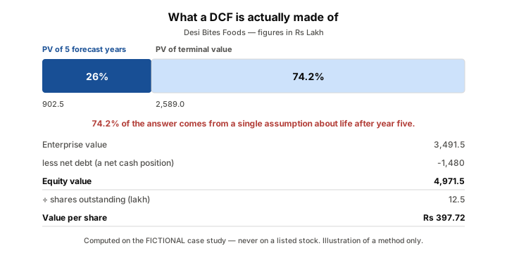
Desi Bites Foods — the fictional case study. The bar shows how much of the valuation rests on the terminal value assumption. Illustration of a method only; this is not a real company and no listed stock is being valued here.

The model disagrees with the market

Desi Bites listed at ₹640. This DCF says ₹397.72 — some 38% below the IPO price.

The tempting move here is to go back and adjust assumptions until the model agrees with the price. Resist it, thoroughly. A model tuned to match a price you already knew has told you nothing you didn’t already know.

The useful move is to run the logic backwards and ask: what would have to be true for ₹640 to be right? Holding the same forecast and the same WACC, that price implies a perpetual growth rate of 9.62% — a claim that Desi Bites keeps pace with the entire Indian economy, forever. That’s right up against the ceiling from the previous section.

Or, keeping terminal growth at 5% and pushing on the operating assumptions instead:

Scenario	Assumptions	Value per share
Base case	Growth fading 18% → 10%, EBITDA margin to 17.5%	₹397.72
Market case	Growth 25% for five years, EBITDA margin 20%, base-case capex path (8% of revenue easing to 5%)	₹595
Aggressive	Growth 30% for five years, EBITDA margin to 22%	₹753

Now the ₹640 price says something specific and testable: it’s priced for sustained 25–30% revenue growth with meaningful margin expansion. Whether that’s optimistic or reasonable is a judgement about the business — but at least it’s a judgement about something concrete, rather than a squabble about whether a stock “looks expensive.”

This is a reverse DCF, and for most people it’s the more useful direction of travel. Forward DCF asks you to produce assumptions and hands you a number. Reverse DCF takes the market’s number and hands you the assumptions hiding inside it — and those assumptions are far easier to argue with.

The calculator

The full model as runnable Python — change the assumptions at the top and everything downstream re-computes:

FY25_REVENUE, TAX, DEP_PCT, NWC_PCT = 2592.0, 0.25, 0.045, 0.0868
WACC, TERMINAL_G = 0.13914, 0.05
NET_DEBT, SHARES = -1480.0, 12.5

growth    = [0.18, 0.16, 0.14, 0.12, 0.10]
margin    = [0.172, 0.174, 0.175, 0.175, 0.175]
capex_pct = [0.08, 0.08, 0.06, 0.05, 0.05]

flows, revenue = [], FY25_REVENUE
for g, m, cx in zip(growth, margin, capex_pct):
    prev, revenue = revenue, revenue * (1 + g)
    dep = revenue * DEP_PCT
    ebit = revenue * m - dep
    flows.append(ebit * (1 - TAX) + dep - revenue * cx - (revenue - prev) * NWC_PCT)

pv_flows = sum(cf / (1 + WACC) ** n for n, cf in enumerate(flows, start=1))
tv = flows[-1] * (1 + TERMINAL_G) / (WACC - TERMINAL_G)
pv_tv = tv / (1 + WACC) ** len(flows)

ev = pv_flows + pv_tv
equity = ev - NET_DEBT
print(f"PV of forecast   {pv_flows:8.1f}")
print(f"PV of terminal   {pv_tv:8.1f}  ({pv_tv / ev:.0%} of EV)")
print(f"Enterprise value {ev:8.1f}")
print(f"Value per share  {equity / SHARES:8.2f}")

Common mistakes

• Not checking what share of the value is terminal. If terminal value is 74.2% of your enterprise value, you have not really valued five years of forecasts — you’ve valued a growth rate in perpetuity, with a five-year preamble. Always compute this percentage. If it’s above about 80%, the forecast horizon is probably too short.
• Setting g too close to WACC. The gap between them is the denominator. Narrow it and the terminal value explodes on arithmetic alone, not on anything you learned about the business.
• Discounting the terminal value by the wrong number of years. It’s n years for an n-year forecast, not n + 1. Off by one here and you cut the terminal value’s contribution by roughly the WACC.
• Getting the net debt sign wrong. Subtract net debt from enterprise value. When the company holds net cash, net debt is negative and you’re subtracting a negative — which adds. Sanity-check the direction every time.
• Using the wrong share count. Use the diluted, post-issue count, as the EPS post covered. Dividing by the pre-IPO count here would have produced ₹497 a share instead of ₹397.72 — a 25% error from one wrong cell.
• Presenting the output as a precise number. ₹397.72 is the arithmetic consequence of a stack of estimates. It is not what the share is worth to two decimal places, and the next post is entirely about why.

Takeaway: Terminal value collapses everything past the forecast horizon into one number, and that number is usually most of the valuation — so the perpetual growth rate deserves more scrutiny than any line in the forecast. And when the model disagrees with the market price, the productive question is never “which is right” but “what is the market assuming that I’m not.”