Seasonality myths, part one: "sell in May" and the best month to invest

The calendar as a trading signal

Every April or May someone repeats it: “Sell in May and go away.” The idea, borrowed from London’s markets, is that stocks do badly from May to October and well from November to April, so you should sit out the summer. Around it sits a lot of other calendar talk about which months are “always” weak or strong.

These claims are called seasonality, or calendar effects. They’re appealing because they’re simple and need no chart at all. They’re also perfect material for the method from the backtesting post: every claim is a fixed-horizon claim (one month, six months), and the data is easy to get.

The research behind the saying is real. Bouman and Jacobsen’s 2002 paper in the American Economic Review reported a “Halloween effect” — better November–April returns — in most of the markets they studied. The question here is narrower: what did the Nifty do?

The formula

Monthly return (month m) = Close on the last trading day of m
                           / Close on the last trading day of m − 1   − 1

For each calendar month, across all years:
   average, median, share of years positive,
   standard deviation (how far a typical year strays from the average),
   worst and best year

Sell in May (year y):
   May–Oct return = Close end-Oct(y) / Close end-Apr(y) − 1
   Nov–Apr return = Close end-Apr(y) / Close end-Oct(y − 1) − 1

The data is the Nifty 50 price index, 17 September 2007 to 30 March 2026, from Yahoo Finance. That gives 222 complete months, October 2007 to March 2026 (March 2026 ends on 30 March, the last row in the file). It’s a price index, so dividends are left out. They add a little to every month and don’t change which month looks best.

Every month, with the spread

Month	Years	Average	Median	Years positive	Std dev	Worst	Best
January	19	−1.3%	−1.7%	26%	6.2%	−16.3%	12.4%
February	19	−1.2%	−0.6%	42%	4%	−7.6%	6.6%
March	19	0.7%	1.6%	63%	8.4%	−23.2%	10.8%
April	18	3%	1.4%	67%	5.3%	−3.6%	15%
May	18	1.8%	1.2%	56%	7.7%	−6.2%	28.1%
June	18	0.7%	1.2%	56%	5.7%	−17%	7.5%
July	18	2.5%	2.5%	72%	4.3%	−5.7%	8.7%
August	18	0%	0.6%	61%	4%	−8.8%	8.7%
September	18	1.1%	0.4%	56%	5.4%	−10.1%	11.6%
October	19	0.8%	1.5%	63%	8.8%	−26.4%	17.5%
November	19	0.6%	−0.3%	47%	5%	−9.3%	11.4%
December	19	1.7%	0.9%	63%	3.8%	−4.3%	7.9%
All months	222	0.9%	0.7%	56%	6%

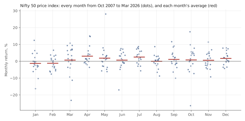
Nifty 50 price index. Source: Yahoo Finance. Historical data, for illustration only.

Read the average column alone and you’d have a story: April is the best month (+3%), January the worst (−1.3%). Now read across to the standard deviation column. A typical month strays from its own average by about 4 to 9 percentage points. The gap between the “best” and “worst” months, 4.3 points, is smaller than that ordinary year-to-year noise in most individual months.

The chart shows why. Each column of dots is one calendar month across roughly 19 years. The red averages sit inside clouds of dots that overlap almost completely, and a single extreme year (the dot far below or above the rest) can drag an average by a point or more.

Is any of that more than chance?

Here’s a simple way to find out. Take all 222 monthly returns, shuffle which calendar month each one belongs to, and recompute the twelve averages. Do that 10,000 times. If the calendar means nothing, how often does the best-minus-worst spread come out at least 4.3 points anyway?

57% of the time. Twelve random buckets of this data usually produce a “best month” and a “worst month” at least that far apart. The month-of-year averages look no more unusual than pure noise would.

One number does look odd. January was positive in only 5 of 19 years (26%). In the same shuffle, the month with the fewest up-years was that bad only 3% of the time. But notice what just happened. We looked at the table, saw January, and then chose a test for it. With twelve months and several ways to rank them (average, median, share positive), something will always look unusual. That’s the parameter-picking problem from the backtesting post, in calendar form. Call it a question worth re-asking on new data, not a finding.

“Sell in May”, year by year

Now the headline claim. For each year, compare the six months from the end of April to the end of October with the six months before it.

Year	Nov–Apr	May–Oct
2008	−12.5%	−44.1%
2009	20.4%	35.6%
2010	12%	14%
2011	−4.5%	−7.4%
2012	−1.5%	7.1%
2013	5.5%	6.2%
2014	6.3%	24.3%
2015	−1.7%	−1.4%
2016	−2.7%	10%
2017	7.7%	11.1%
2018	3.9%	−3.3%
2019	13.1%	1.1%
2020	−17%	18.1%
2021	25.7%	20.8%
2022	−3.2%	5.3%
2023	0.3%	5.6%
2024	18.5%	7.1%
2025	0.5%	5.7%

The first row is November 2007–April 2008 against May–October 2008. The November 2025–April 2026 window is left out, because the data ends 30 March 2026.

Over these 18 years:

Item	Nov–Apr	May–Oct
Average	3.9%	6.4%
Median	2.2%	6.7%

On the Nifty, the “go away” months were the better half on average, and May–October was positive in 14 of 18 years. It beat the November–April half in 12 of them. Selling every May would mostly have meant sitting out rising markets. And you’d also have paid costs twice a year, and tax on any gains you realised.

That doesn’t prove the opposite rule works either. The biggest single number in the table, a May–October fall of 44.1% in 2008, came from the global financial crisis, not from the calendar. Eighteen six-month windows are too few to say any half of the year is reliably better.

🧒 Explain it like I'm 10 (optional — skip if this is already clear)

Imagine rolling a dice twelve times and writing each roll under a month name. One month will get the biggest number and one the smallest. That doesn’t mean the dice likes March.

Do it again next year and a different month wins. If you want to know whether a month is really special, you check whether it keeps winning, year after year, by more than the dice would give it anyway. For the Nifty, it mostly doesn’t.

Doing it in Python

import pandas as pd

s = pd.read_csv("nifty50-price-index.csv", parse_dates=["date"]
                ).set_index("date").nifty50_pri_close

m = s.resample("ME").last().pct_change().dropna() * 100
m = m["2007-10":]                       # first complete month
by = m.groupby(m.index.month)
print(pd.DataFrame({"avg": by.mean(), "median": by.median(),
                    "up%": by.apply(lambda x: (x > 0).mean() * 100),
                    "std": by.std(), "n": by.size()}).round(1))

# shuffle test: how often do random month labels give as wide a spread?
real = by.mean().max() - by.mean().min()
wider = sum((g := m.groupby(m.sample(frac=1, random_state=i).index.month).mean()
             ).max() - g.min() >= real for i in range(2000))
print(f"spread {real:.1f} pts; random labels as wide {wider / 2000:.0%} of the time")

The shuffle line works because m.sample(frac=1) reorders the values while .index.month on the shuffled series still hands each value a random month label. Your percentage will wobble a point or two from ours, because the shuffles are random.

Common mistakes

• Reading averages without the spread. An average of +3% with a standard deviation of 5% says “most Aprils were somewhere between −2% and +8%”. That’s not a forecast; it’s a wide range.
• Letting one year drive the story. Monthly averages over 18–19 years shift noticeably when you add or drop a single crisis year. Check the median and the share of positive years too.
• Finding a pattern, then testing the pattern you found. The January result above is exactly this. A test chosen after looking at the data tends to pass more often than it should.
• Ignoring the cost of acting on it. A calendar rule trades on fixed dates regardless of anything else. Each switch costs brokerage, taxes and slippage, and those are certain, while the calendar edge is not.

Takeaway: On the Nifty since 2007, “sell in May” would mostly have meant missing rising markets: May–October was the better half on average. Month-by-month averages look like a pattern, but shuffling the month labels produces spreads that wide more often than not.