Bollinger Bands and ATR: measuring volatility, not direction

A different question

Everything in the first ten posts of this series asked some version of which way? Trend lines, moving averages, RSI, MACD — all of them are, at bottom, attempts to read direction.

This post asks a different and more answerable question: how much does this thing move? That is volatility, and two of the most common tools for measuring it — Bollinger Bands and the Average True Range — are useful precisely because they don’t pretend to know direction. They tell you how wide the road is, not which way the car is going.

Same dataset as the rest of the series: Britannia (NSE: BRITANNIA), daily bars, 1 April 2024 to 30 March 2026. The data ends 30 March 2026, about 6 months before this post — well past the three-month lag this blog keeps on every real price series.

Bollinger Bands: the formula

Take a moving average, then draw a line two standard deviations above it and two below:

Middle band  = SMA(20)
Upper band   = SMA(20) + 2 × σ(20)
Lower band   = SMA(20) − 2 × σ(20)

σ(20) = population standard deviation of the last 20 closes

Bandwidth  = (Upper − Lower) / Middle               how wide are they?

The standard deviation is the whole idea. When price has been jumping around, σ is large and the bands are wide; when it has been quiet, σ shrinks and the bands pinch together. The bands are a volatility ruler drawn around a moving average.

You’ll often read that about 95% of closes should fall inside the bands, because 95% of random draws from a normal distribution land within two standard deviations. That rule is for independent draws around a fixed average. Bollinger’s σ is measured on the last 20 closing prices — levels, not daily returns — and prices trend. Each close sits near the one before, so in a steady move the whole window drifts and the newest close keeps landing near the edge, or past it. In this dataset 86.1% of closes sat inside the bands. Treat the 95% as a loose analogy, not a probability.

🧒 Explain it like I'm 10 (optional — skip if this is already clear)

Imagine walking a dog on a lead that stretches. When the dog is calm, it stays close and the lead is slack — the “band” around you is narrow. When the dog is excited, it darts about and the lead stretches to its limit in every direction.

Bollinger Bands are that lead, drawn around the price. Wide bands mean the dog has been darting. Narrow bands mean it’s been calm. Neither tells you which way the dog will run next — only how far it’s been running lately.

The chart

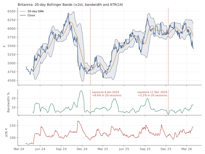
Britannia (NSE: BRITANNIA), daily bars, 1 April 2024 to 30 March 2026. Source: Yahoo Finance. Historical data, for illustration only.

Three panels: price with the bands, the bandwidth underneath, and the ATR at the bottom. Notice how the bands bulge during the late-2024 decline and pinch in the quiet stretches. Bandwidth ranged from 2.5% (11 December 2025) to 28.4% (28 November 2024) — an elevenfold difference in how much the same stock was moving, over 24 months.

The two readings people take from the bands

1. “Price touched the upper band, so it’s overbought.” This is the common reading and mostly a mistake. A close above the upper band means price moved more than two standard deviations from its average — which happens most often during strong trends, when it keeps happening. In this dataset:

Event	Count	With 10 sessions of data after	Average return over the next 10 sessions	Share positive
Close above the upper band	43	43	0.92%	60.5%
Close below the lower band	23	20	−0.41%	50.0%

Events too close to the end of the data to have ten sessions after them are left out of the averages and shares.

Read that carefully. After a close above the upper band, the stock was on average slightly higher ten days later, not lower. After a close below the lower band, it was on average slightly lower, and it finished higher only 50.0% of the time — a coin flip, not a bounce. The “reversal” reading points the wrong way in this sample — the same pinned-in-a-trend problem the RSI post documented. That’s 63 scored events on one stock, so treat it as an illustration, not a law. But it is not evidence for the reversal reading.

2. “The bands are pinching — a big move is coming.” This is the squeeze, and it is the more defensible use, because it’s a statement about volatility rather than direction. Volatility clusters — quiet days tend to follow quiet days, and loud days follow loud ones — but over longer stretches it drifts back toward its usual level. So an unusually quiet spell can’t last forever, and when it ends, the moves get bigger. Whether up or down is not part of the claim.

Two squeezes in this dataset, defined as bandwidth hitting a 120-session low:

Squeeze	Bandwidth	Close	20 sessions later	Move
2025-01-06	3.8%	₹4,791.2	₹5,201.4 (2025-02-01)	+8.6%
2025-12-11	2.5%	₹5,847	₹5,977.5 (2026-01-09)	+2.2%

The January 2025 squeeze was followed by a 8.6% move in four weeks — the kind of chart that ends up in a tutorial. The December 2025 squeeze was tighter — the narrowest bands in the whole two years — and resolved into 2.2%, which is an ordinary month. Same setup, tighter reading, nothing much happened.

One honesty note: each row is dated to the last session of its squeeze, the day the bands were tightest — which you could only know afterwards. Measured from the first session of each squeeze (3 January 2025 and 8 December 2025), the 20-session moves were +6.1% and +4.8% — much closer together, which makes the same point less dramatically.

That is the honest shape of the squeeze: it raises the odds of a large move without promising one, and it says nothing at all about direction.

ATR: the formula

ATR — Average True Range — answers the simplest volatility question there is: on a typical day, how many rupees does this stock travel?

True Range (TR) = max( High − Low,
                       |High − Previous Close|,
                       |Low  − Previous Close| )

ATR(14) = Wilder-smoothed average of TR over 14 sessions
          (α = 1/14, the same smoothing RSI uses)

Why “true” range rather than just high minus low? Because of gaps. If a stock closes at 5,000 and opens the next morning at 4,850, the day’s high–low range might be tiny while the actual move from yesterday was 150. True range counts that gap.

For Britannia, ATR ranged from ₹73.6 (3 May 2024) to ₹169.4 (12 November 2024), and the median was about 2.08% of the price. So on an ordinary day this stock travelled roughly 2% of its value — a number worth knowing before deciding how far away a stop-loss belongs.

What ATR is actually for: sizing a stop

This is the genuinely practical use, and it’s about risk management rather than prediction. A stop-loss placed “5% below” is arbitrary — 5% is nothing for a volatile small-cap and a lot for a staid large-cap. A stop placed two ATRs below adapts to the stock’s own behaviour.

Worked on a historical date — 4 June 2025, the golden-cross day from the moving-averages post, chosen for continuity, not as a signal:

Item
Close	₹5,542
ATR(14)	₹111.7
Stop at 2 × ATR below	₹5,318.5 (4.0% away)
Risk budget (illustrative: 2% of a ₹1,00,000 account)	₹2,000
Shares such that a stop-out loses the budget	₹2,000 ÷ (2 × ₹111.7) = 8
Lowest low over the next 20 sessions	₹5,425
Stop hit?	No

The chain is: the stock’s volatility sets the stop distance, the stop distance plus a fixed rupee risk sets the position size. Volatile stock → wider stop → fewer shares. That is the entire logic of ATR-based position sizing, and the risk series on this blog builds a whole post on it. Here, the point is only that ATR turns “how far away should my stop be?” from a guess into a measurement.

Doing it in Python

import pandas as pd

df = pd.read_csv("britannia-ohlcv-2024-04-to-2026-03.csv",
                 parse_dates=["date"]).set_index("date")

# Bollinger Bands: 20-day SMA ± 2 population std devs
mid = df.close.rolling(20).mean()
sd  = df.close.rolling(20).std(ddof=0)        # ddof=0: population, as Bollinger specified
df["upper"], df["lower"] = mid + 2*sd, mid - 2*sd
df["bandwidth"] = (df.upper - df.lower) / mid * 100

# ATR(14), Wilder smoothing
prev = df.close.shift()
tr = pd.concat([df.high - df.low,
                (df.high - prev).abs(),
                (df.low - prev).abs()], axis=1).max(axis=1)
df["atr"] = tr.ewm(alpha=1/14, adjust=False).mean()

print(df[["close", "bandwidth", "atr"]].iloc[20:].describe().round(1))

ddof=0 matters. pandas defaults to the sample standard deviation (ddof=1), which gives slightly wider bands than most charting software. Neither is “wrong”, but if your numbers don’t match your broker’s chart, this is usually why.

Common mistakes

• Reading a band touch as a reversal signal. In this dataset closes above the upper band were followed, on average, by further gains. In a trend, price walks the band.
• Reading a squeeze as directional. The squeeze says “a bigger move is more likely.” It does not say which way, and the tightest squeeze in two years was followed by very little.
• Using a fixed-percentage stop on every stock. 5% is two and a half ATRs for this stock and might be half an ATR for a volatile small-cap. Let the stock’s own range set the distance.
• Placing the stop exactly at 2 × ATR because a post said so. Two is a convention. The principle is scale to volatility; the multiplier is a choice you should be able to defend.
• Forgetting the warmup. The first 20 bandwidth values and the first ~14 ATR values are not real readings.

Takeaway: Bollinger Bands and ATR measure how much a stock moves, not where it’s going — and they’re most useful when you let them stay in that lane. On two years of Britannia, closes above the upper band were followed by gains more often than falls, the tightest squeeze of the period resolved into an ordinary month, and the one thing ATR reliably did was turn “how far away should my stop be?” into a number.